Multi-processing in Julia

Table of contents

Thursday, October 14, 2021
2:00pm - 4:00pm

In a Research Commons workshop in May, we gave a quick introduction to parallel programming in Julia. For heavy computations, Julia supports multiple threads and multiprocessing, both via the Standard Library and via a number of external packages. Today we will spend more time on Julia multiprocessing with Distributed.jl, walking participants through a series of hands-on exercises where you launch processes either on the same multi-core machine or on a multi-node HPC cluster.

Prerequisites: We expect participants to be somewhat familiar with basic Julia syntax and with running Julia codes interactively – this material was covered in our introductory webinar https://bit.ly/2Y8LJbZ. For all participants, we will provide access (with guest accounts) to a remote cluster with Julia installed, so you don’t need to install Julia on your computer (although you can via https://julialang.org/downloads). To access our remote system, you will need to install an SSH client on your computer such as the free MobaXterm Home Edition from https://mobaxterm.mobatek.net/download.html.

Processes vs. threads

In Unix a process is the smallest independent unit of processing, with its own memory space – think of an instance of a running application. The operating system tries its best to isolate processes so that a problem with one process doesn’t corrupt or cause havoc with another process. Context switching between processes is relatively expensive.

A process can contain multiple threads, each running on its own CPU core (parallel execution), or sharing CPU cores if there are too few CPU cores relative to the number of threads (parallel + concurrent execution). All threads in a Unix process share the virtual memory address space of that process, e.g. several threads can update the same variable, whether it is safe to do so or not. Context switching between threads of the same process is less expensive.

$Image copied from\nhttps://www.backblaze.com/blog/whats-the-diff-programs-processes-and-threads$

Threads within a process communicate via shared memory, so multi-threading is always limited to shared memory within one node.
Processes communicate via messages (over the cluster interconnect or via shared memory). Multi-processing can be in shared memory (one node, multiple CPU cores) or distributed memory (multiple cluster nodes). With multi-processing there is no scaling limitation, but traditionally it has been more difficult to write code for distributed-memory systems. Julia tries to simplify it with high-level abstractions.

In Julia you can parallelize your code with multiple threads, or with multiple processes, or both (hybrid parallelization).

Discussion

What are the benefits of each: threads vs. processes? Consider (1) context switching, e.g. starting and terminating or concurrent execution, (2) communication, (3) scaling up.

Running Julia in REPL

If you have Julia installed on your own computer, you can run it there. We have Julia on our training cluster uu.c3.ca. In our introductory Julia course we were using Julia inside a Jupyter notebook. Today we will be running multiple threads and processes, with the eventual goal of running our workflows as batch jobs on an HPC cluster, so we’ll be using Julia from the command line.

Pause: We will now distribute accounts and passwords to connect to the cluster.

Our training cluster has:

one login node with 16 “persistent” cores and 32GB memory, and
16 compute nodes with 2 “compute” cores and 7.5GB memory each.

Julia packages on the training cluster

Normally, you would install a Julia package by typing ] add packageName in REPL and then waiting for it to install. A typical package installation takes few hundred MBs and a fraction of a minute and usually requires a lot of small file writes. Our training cluster runs on top of virtualized hardware with a shared filesystem. If several dozen workshop participants start installing packages at the same time, this will hammer the filesystem and will make it slow for all participants for quite a while.

To avoid this, we created a special environment, with all packages installed into a shared directory /project/def-sponsor00/shared/julia. To load this environment, run the command

source /project/def-sponsor00/shared/julia/config/loadJulia.sh

This script will load the Julia module and set a couple of environment variables, to point to our central environment while keeping your setup and Julia history separate from other users. You can still install packages the usual way (] add packageName), and they will go into your own ~/.julia directory. Feel free to check the content of this script, if you are interested.

Try opening the Julia REPL and running a couple of commands:

$ julia 
               _
   _       _ _(_)_     |  Documentation: https://docs.julialang.org
  (_)     | (_) (_)    |
   _ _   _| |_  __ _   |  Type "?" for help, "]?" for Pkg help.
  | | | | | | |/ _` |  |
  | | |_| | | | (_| |  |  Version 1.6.2 (2021-07-14)
 _/ |\__'_|_|_|\__'_|  |  
|__/                   |

julia> using BenchmarkTools

julia> @btime sqrt(2)
  1.825 ns (0 allocations: 0 bytes)
1.4142135623730951

Benchmarking in Julia

We can use @time macro for timing our code. Let’s do summation of integers from 1 to Int64(1e8) using a serial code:

n = Int64(1e8)
total = Int128(0)   # 128-bit for the result!
@time for i in 1:n
	global total += i
end
println("total = ", total)

On Uu I get 10.87s, 10.36s, 11.07s. Here @time also includes JIT compilation time (marginal here). Let’s switch to @btime from BenchmarkTools: it runs the code several times, reports the shortest time, and prints the result only once. Therefore, with @btime you don’t need to precompile the code.

using BenchmarkTools
n = Int64(1e8)
total = Int128(0)   # 128-bit for the result!
@btime for i in 1:n
	global total += i
end
println("total = ", total)

10.865 s

Next we’ll package this code into a function:

function quick(n)
    total = Int128(0)   # 128-bit for the result!
    for i in 1:n
        total += i
    end
    return(total)
end

@btime quick(Int64(1e8))    # correct result, 1.826 ns runtime
@btime quick(Int64(1e9))    # correct result, 1.825 ns runtime
@btime quick(Int64(1e15))   # correct result, 1.827 ns runtime

In all these cases we see under 2 ns running time – this can’t be correct! What is going on here? It turns out that Julia is replacing the summation with the exact formula $n (n + 1) / 2$ !

We want to:

force computation $\Rightarrow$ we’ll compute something more complex than simple integer summation, so that it cannot be replaced with a formula
exclude compilation time $\Rightarrow$ we’ll package the code into a function + precompile it
make use of optimizations for type stability $\Rightarrow$ package into a function + precompile it
time only the CPU-intensive loops

Slowly convergent series

We could replace integer summation $~~\sum_{i=1}^\infty i~~ $w i t h t h e h a r m o n i c s e r i e s, h o w e v e r, t h e t r a d i t i o n a l h a r m o n i c s e r i e s$ ~~\sum\limits_{k=1}^\infty{1\over k}~~$ diverges. It turns out that if we omit the terms whose denominators in decimal notation contain any digit or string of digits, it converges, albeit very slowly (Schmelzer & Baillie 2008), e.g.

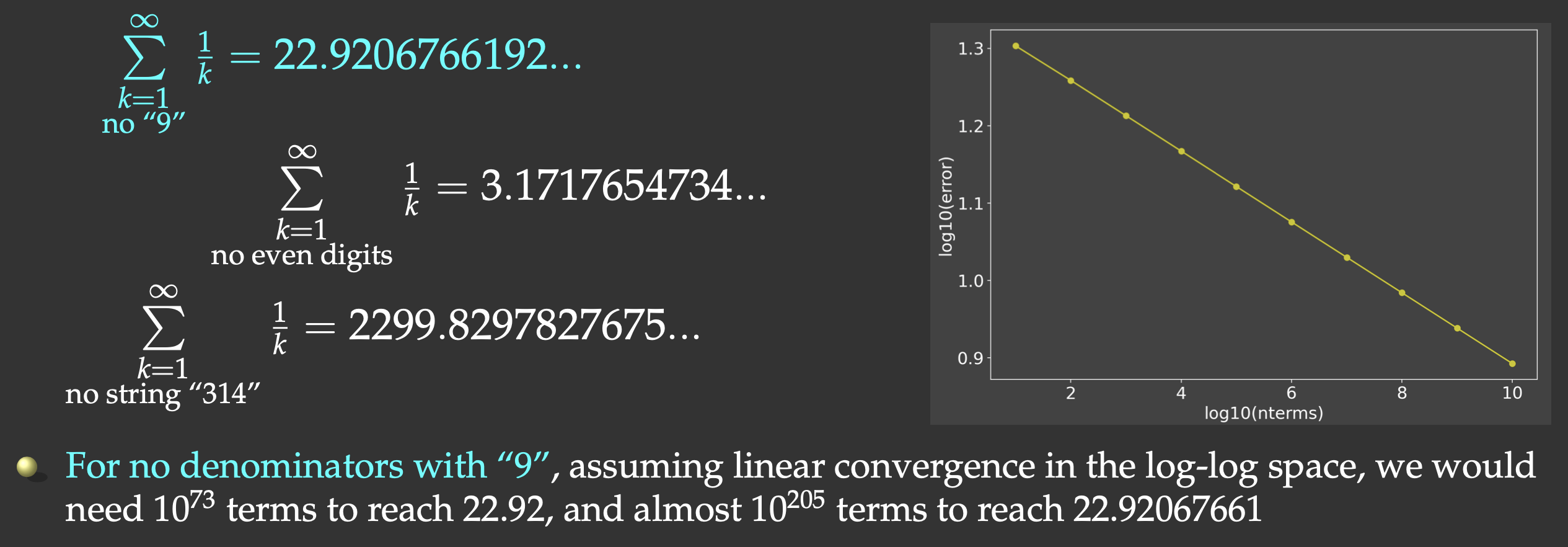
But this slow convergence is actually good for us: our answer will be bounded by the exact result (22.9206766192…) on the upper side. We will sum all the terms whose denominators do not contain the digit “9”.

We will have to check if “9” appears in each term’s index i. One way to do this would be checking for a substring in a string:

if !occursin("9", string(i))
    <add the term>
end

It turns out that integer exclusion is ∼4X faster (thanks to Paul Schrimpf from the Vancouver School of Economics @UBC for this code!):

function digitsin(digits::Int, num)   # decimal representation of `digits` has N digits
    base = 10
    while (digits ÷ base > 0)   # `digits ÷ base` is same as `floor(Int, digits/base)`
        base *= 10
    end
    # `base` is now the first Int power of 10 above `digits`, used to pick last N digits from `num`
    while num > 0
        if (num % base) == digits     # last N digits in `num` == digits
            return true
        end
        num ÷= 10                     # remove the last digit from `num`
    end
    return false
end
if !digitsin(9, i)
    <add the term>
end

Let’s now do the timing of our serial summation code with 1e9 terms:

function slow(n::Int64, digits::Int)
    total = Float64(0)    # this time 64-bit is sufficient!
    for i in 1:n
        if !digitsin(digits, i)
            total += 1.0 / i
        end
	end
    return total
end
@btime slow(Int64(1e8), 9)   # total = 13.277605949858103, runtime 2.986 s

Distributed.jl

Julia’s Distributed package provides multiprocessing environment to allow programs to run on multiple processors in shared or distributed memory. On each CPU core you start a separate Unix / MPI process, and these processes communicate via messages. Unlike traditionally in MPI, Julia’s implementation of message passing is one-sided, typically with higher-level operations like calls to user functions on a remote process.

a remote call is a request by one processor to call a function on another processor; returns a remote/future reference
the processor that made the call proceeds to its next operation while the remote call is computing, i.e. the call is non-blocking
you can obtain the remote result with fetch() or make the calling processor block with wait()

In this workflow you have a single control process + multiple worker processes. Processes pass information via messages underneath, not via variables in shared memory

Launching worker processes

There are three different ways you can launch worker processes:

with a flag from bash:

julia -p 8             # open REPL, start Julia control process + 8 worker processes
julia -p 8 code.jl     # run the code with Julia control process + 8 worker processes

from a job submission script:

#!/bin/bash
#SBATCH --ntasks=8
#SBATCH --cpus-per-task=1
#SBATCH --mem-per-cpu=3600M
#SBATCH --time=00:10:00
#SBATCH --account=def-someuser
srun hostname -s > hostfile   # parallel I/O
sleep 5
module load julia/1.6.0
julia --machine-file ./hostfile ./code.jl

from the control process, after starting Julia as usual with julia:

using Distributed
addprocs(8)

Note: All three methods launch workers, so combining them will result in 16 (or 24!) workers (probably not the best idea). Select one method and use it.

In Slurm methods (1) and (3) work very well, so - when working on a CC cluster - usually there is no need to construct a machine file.

Process control

Let’s restart Julia with julia (single control process).

using Distributed
addprocs(4)   # add 4 worker processes; this might take a while on Uu
println("number of cores = ", nprocs())       # 5 cores
println("number of workers = ", nworkers())   # 4 workers
workers()                                     # list worker IDs

You can easily remove selected workers from the pool:

rmprocs(2, 3, waitfor=0)   # remove processes 2 and 3 immediately
workers()

or you can remove all of them:

for i in workers()     # cycle through all workers
    t = rmprocs(i, waitfor=0)
    wait(t)            # wait for this operation to finish
end
workers()
interrupt()   # will do the same (remove all workers)
addprocs(4)   # add 4 new worker processes (notice the new IDs!)
workers()

Discussion

If from the control process we start $N = 8$ workers, where will these processes run? Consider the following cases:

a laptop with 2 CPU cores,

a cluster login node with 16 CPU cores,

a cluster Slurm job with 4 CPU cores.

Remote calls

Let’s restart Julia with julia (single control process).

using Distributed
addprocs(4)       # add 4 worker processes

Let’s define a function on the control process and all workers and run it:

@everywhere function showid()   # define the function everywhere
    println("my id = ", myid())
end
showid()                        # run the function on the control process
@everywhere showid()            # run the function on the control process + all workers

@everywhere does not capture any local variables (unlike @spawnat that we’ll study below), so on workers we don’t see any variables from the control process:

x = 5     # local (control process only)
@everywhere println(x)    # get errors: x is not defined elsewhere

However, you can still obtain the value of x from the control process by using this syntax:

@everywhere println($x)   # use the value of `x` from the control process

The macro that we’ll use a lot today is @spawnat. If we type:

a = 12
@spawnat 2 println(a)     # will print 12 from worker 2

it will do the following:

pass the namespace of local variables to worker 2
spawn function execution on worker 2
return a Future handle (referencing this running instance) to the control process
return REPL to the control process (while the function is running on worker 2), so we can continue running commands

Now let’s modify our code slightly:

a = 12
@spawnat 2 a+10          # Future returned but no visible calculation

There is no visible calculation happening; we need to fetch the result from the remote function before we can print it:

r = @spawnat 2 a+10
typeof(r)
fetch(r)                 # get the result from the remote function; this will pause
                         #         the control process until the result is returned

You can combine both @spawnat and fetch() in one line:

fetch(@spawnat 2 a+10)   # combine both in one line; the control process will pause
@fetchfrom 2 a+10        # shorter notation; exactly the same as the previous command

Exercise “Distributed.1”

Try to define and run a function on one of the workers, e.g.
function cube(x)
    return x*x*x
end

Exercise “Distributed.2”

Now run the same function on all workers, but not on the control process. Hint: use workers() to cycle through all worker processes.

You can also spawn computation on any available worker:

r = @spawnat :any log10(a)   # start running on one of the workers
fetch(r)

Back to the slow series: serial code

Let’s restart Julia with julia -p 2 (control process + 2 workers). We’ll start with our serial code (below), and let’s save it as serialDistributed.jl and run it.

using Distributed
using BenchmarkTools

@everywhere function digitsin(digits::Int, num)
    base = 10
    while (digits ÷ base > 0)
        base *= 10
    end
    while num > 0
        if (num % base) == digits
            return true
        end
        num ÷= 10
    end
    return false
end

@everywhere function slow(n::Int64, digits::Int)
    total = Int64(0)
    for i in 1:n
        if !digitsin(digits, i)
            total += 1.0 / i
        end
    end
    return total
end

@btime slow(Int64(1e8), 9)     # serial run: total = 13.277605949858103

For me this serial run takes 2.997 s on Uu’s login node. Next, let’s run it on 3 (control + 2 workers) cores simultaneously:

@everywhere using BenchmarkTools
@everywhere @btime slow(Int64(1e8), 9)   # runs on 3 (control + 2 workers) cores simultaneously

Here we are being silly: this code is serial, so each core performs the same calculation … I see the following times printed on my screen: 3.097 s, 2.759 s, 3.014 s – each is from a separate process running the code in serial.

How do we make this code parallel and make it run faster?

Parallelizing our slow series: non-scalable version

Let’s restart Julia with julia (single control process) and add 2 worker processes:

using Distributed
addprocs(2)
workers()

We need to redefine digitsin() everywhere, and then let’s modify slow() to compute a partial sum:

@everywhere function slow(n::Int, digits::Int, taskid, ntasks)   # two additional arguments
    println("running on worker ", myid())
    total = 0.
    @time for i in taskid:ntasks:n   # partial sum with a stride `ntasks`
        if !digitsin(digits, i)
            total += 1. / i
        end
    end
    return(total)
end

Now we can actually use it:

# slow(Int64(10), 9, 1, 2)   # precompile the code
precompile(slow, (Int, Int, Int, Int))
a = @spawnat :any slow(Int64(1e8), 9, 1, 2)
b = @spawnat :any slow(Int64(1e8), 9, 2, 2)
print("total = ", fetch(a) + fetch(b))   # 13.277605949852546

For timing I got 1.26s and 1.31s, running concurrently, which is a 2X speedup compared to the serial run – this is great result! Notice that we received a slightly different numerical result, due to a different order of summation.

However, our code is not scalable: it’s only limited to a small number of sums each spawned with its own Future reference. If we want to scale it to 100 workers, we’ll have a problem.

How do we solve this problem – any ideas before I show the solution in the next section?

Solution 1: an array of Future references

We could create an array (using array comprehension) of Future references and then add up their respective results. An array comprehension is similar to Python’s list comprehension:

a = [i for i in 1:5];   # array comprehension in Julia
typeof(a)               # 1D array of Int64

We can cycle through all available workers:

[w for w in workers()]                      # array of worker IDs
[(i,w) for (i,w) in enumerate(workers())]   # array of tuples (counter, worker ID)

Exercise “Distributed.3”

Using this syntax, construct an array r of Futures, and then get their results and sum them up with
print("total = ", sum([fetch(r[i]) for i in 1:nworkers()]))
You can do this exercise using either the array comprehension from above, or the good old for loops.

With two workers and two CPU cores, we should get times very similar to the last run. However, now our code can scale to much larger number of cores!

Exercise “Distributed.4”

If you did the previous exercise on the login node, now submit a Slurm job running the same code on two full Uu nodes (4 CPU cores). If you did the previous exercise with Slurm, now change the number of workers. Did your timing change?

Solution 2: parallel `for` loop with summation reduction

Unlike Base.Threads module, Distributed provides a parallel loop with reduction. This means that we can implement a parallel loop for computing the sum. Let’s write parallelFor.jl with this version of the function:

function slow(n::Int64, digits::Int)
    @time total = @distributed (+) for i in 1:n
        !digitsin(digits, i) ? 1.0 / i : 0
    end
    println("total = ", total);
end

A couple of important points:

We don’t need @everywhere to define this function. It is a parallel function defined on the control process, and running on the control process.
The only expression inside the loop is the compact if/else statement. Consider this:

1==2 ? println("Yes") : println("No")

The outcome of the if/else statement is added to the partial sums at each loop iteration, and all these partial sums are added together.

Now let’s measure the times:

# slow(10, 9)
precompile(slow, (Int, Int))
slow(Int64(1e8), 9)   # total = 13.277605949855722

Exercise “Distributed.5”

Switch from using @time to using @btime in this code. What changes did you have to make?

This will produce the single time for the entire parallel loop (1.498s in my case).

Exercise “Distributed.6”

Repeat on four full Uu nodes (8 CPU cores). Did your timing improve?

I tested this code (parallelFor.jl) on Cedar with v1.5.2 and n=Int64(1e9):

#!/bin/bash
#SBATCH --ntasks=...   # number of MPI tasks
#SBATCH --cpus-per-task=1
#SBATCH --nodes=1-1   # change process distribution across nodes
#SBATCH --mem-per-cpu=3600M
#SBATCH --time=0:5:0
#SBATCH --account=...
module load julia
echo $SLURM_NODELIST
# comment out addprocs() in the code
julia -p $SLURM_NTASKS parallelFor.jl

Code	Time
serial	48.2s
4 cores, same node	12.2s
8 cores, same node	7.6s
16 cores, same node	6.8s
32 cores, same node	2.0s
32 cores across 6 nodes	11.3s

Solution 3: use `pmap` to map arguments to processes

Let’s write mappingArguments.jl with a new version of slow() that will compute partial sum on each worker:

@everywhere function slow((n, digits, taskid, ntasks))   # the argument is now a tuple
    println("running on worker ", myid())
	total = 0.0
	@time for i in taskid:ntasks:n   # partial sum with a stride `ntasks`
        !digitsin(digits, i) && (total += 1.0 / i)   # compact if statement
    end
    return(total)
end

and launch the function on each worker:

slow((10, 9, 1, 1))   # package arguments in a tuple
nw = nworkers()
args = [(Int64(1e8),9,j,nw) for j in 1:nw]   # array of tuples to be mapped to workers
println("total = ", sum(pmap(slow, args)))   # launch the function on each worker and sum the results

These two syntaxes are equivalent:

sum(pmap(slow, args))
sum(pmap(x->slow(x), args))

We see the following times from individual processes:

From worker 2:	running on worker 2
From worker 3:	running on worker 3
From worker 4:	running on worker 4
From worker 5:	running on worker 5
From worker 2:	  0.617099 seconds
From worker 3:	  0.619604 seconds
From worker 4:	  0.656923 seconds
From worker 5:	  0.675806 seconds
total = 13.277605949854518

Processes vs. threads

Discussion

Running Julia in REPL

Julia packages on the training cluster

Benchmarking in Julia

Slowly convergent series

Distributed.jl

Launching worker processes

Process control

Discussion

Remote calls

Exercise “Distributed.1”

Exercise “Distributed.2”

Back to the slow series: serial code

Parallelizing our slow series: non-scalable version

Solution 1: an array of Future references

Exercise “Distributed.3”

Exercise “Distributed.4”

Solution 2: parallel for loop with summation reduction

Exercise “Distributed.5”

Exercise “Distributed.6”

Solution 3: use pmap to map arguments to processes

Solution 2: parallel `for` loop with summation reduction

Solution 3: use `pmap` to map arguments to processes