Setup and running Jupyter notebooks
Disclaimer: These notes started few years ago from the official SWC lesson but then evolved quite a bit to include other topics.
Why Python?
Python is a free, open-source programming language developed in the 1980s and 90s that became really popular for scientific computing in the past 15 years.
Python vs. Excel
- Unlike Excel, Python can essentially read any type of data, both structured and unstructured.
- Python is free and open-source.
- Data manipulation is much easier in Python. There are thousands of data processing, machine learning, and visualization libraries.
- Python can handle much larger amounts of data: limited not by Python, but by your available computing resources. In addition, Python can run at scale on larger systems.
- Python is more reproducible (rerun / modify the script).
- Python can run on any platform (Windows, Mac, Linux).
Python vs. other programming languages
| Python pros | Python cons |
|---|---|
| elegant scripting language | slow (interpreted, dynamically typed) |
| powerful, compact constructs for many tasks | |
| very popular across all fields | |
| huge number of external libraries |
Starting Python
There are many ways to run Python commands:
- from a Unix shell you can start a Python shell and type commands there,
- you can launch Python scripts saved in plain text *.py files,
- you can execute Python cells inside Jupyter notebooks; the code is stored inside JSON files, displayed as HTML
Today’s options:
- Local option: if you have Python + Jupyter installed locally on your computer, and you know what you
are doing, you can start a Jupyter notebook locally in your browser by typing
jupyter notebookorjupyter labin your shell. For this to work, you will need to installjupyterorjupyterlab(see below).- Local method 1: (1) Install Python from https://www.python.org/downloads, (2) make sure to check the
option “Add Python to PATH” during the installation, (3) install Jupyter Notebook via the Command Prompt
pip install jupyter, and then (4) launch Jupyter Notebook viajupyter notebook. - Local method 2: Install Python and the packages via Anaconda from https://www.anaconda.com/download.
- Local method 1: (1) Install Python from https://www.python.org/downloads, (2) make sure to check the
option “Add Python to PATH” during the installation, (3) install Jupyter Notebook via the Command Prompt
For the extended version of this workshop (covering Scientific Python) you will also need the following Python
packages installed on your computer: numpy, matplotlib, pandas, scikit-image, xarray,
nc-time-axis, netcdf4.
Installing packages locally can be tricky – details depend on the OS and your preferred Python installation
method. For example, as of September 2023, if you are on a Mac and install Python via Homebrew, you will need
to downgrade your jupyterlab to avoid a bug in Homebrew:
pip uninstall jupyterlab
pip install jupyterlab==3.6.3
jupyter lab build
jupyter notebook   # or `jupyter lab`
- Remote option: You can run Python in the command line inside an interactive job on our training cluster
(important: do not run Python on the login node). To do this, log in to
oc.c3.cavia SSH and start a serial interactive job:
$ salloc --time=03:00:00 --mem=3600
$ source ~/projects/def-sponsor00/shared/astro/bin/activate
$ python
Python 3.8.10 (default, Jun 16 2021, 14:20:20)
[GCC 9.3.0] on linux
Type "help", "copyright", "credits" or "license" for more information.
>>> import numpy as np
>>> np.sqrt(2)
Working in the terminal, you won’t have access to all the bells and whistles of the Jupyter interface, and you will have to plot matplotlib graphics into remote PNG files and then download them to view locally on your computer. On the other hand, this option most closely resembles working in the terminal on a remote HPC cluster.
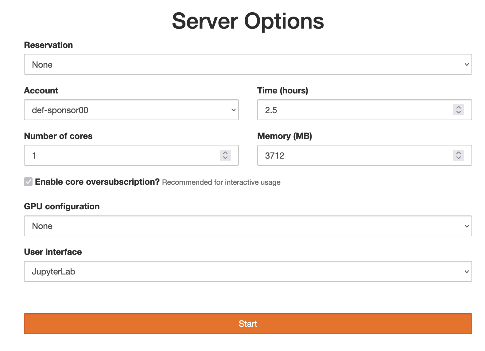
- Remote option is the GUI version of the previous option: use JupyterHub on our training cluster. Point your browser to https://oc.c3.ca, log in with your username and password, then launch a JupyterHub server with time = 4 hours, 1 CPU core, memory = 3600 MB, GPU configuration = None, user interface = JupyterLab. Finally, start a new Python 3 notebook.
- Community cloud option: use syzygy.ca with one of the following accounts:
- if you have a university computer ID → go to syzygy.ca, under Launch select your institution, then log in with your university credentials
- if you have a Google account → go to syzygy.ca, under Launch select either Cybera or PIMS, then log in with your Google account
After you log in, start a new Python 3 notebook.
Note that syzygy.ca is a free community service run on the Alliance cloud and used heavily for undergraduate teaching, with no uptime guarantees. In other words, it usually works, but it could be unstable or down.
Virtual Python environments
We talk about creating Virtual Python environments in the HPC course. These environment are very useful, as not only can you install packages into your directories without being root, but they also let you create sandbox Python environments with your custom set of packages – perfect when you work on multiple projects, each with a different list of dependencies.
To create a Python environment (you do this only once):
module avail python               # several versions available
module load python/3.10.2
virtualenv --no-download astro    # install Python tools in your $HOME/astro
source astro/bin/activate
pip install --no-index --upgrade pip
pip install --no-index numpy jupyter pandas            # all these will go into your $HOME/astro
avail_wheels --name "*tensorflow_gpu*" --all_versions   # check out the available packages
pip install --no-index tensorflow_gpu==2.2.0            # if needed, install a specific version
...
deactivate
Once created, you would use it with:
source ~/astro/bin/activate
python
...
deactivate
We’ll talk more about virtual Python environments in Section 10.
Navigating Jupyter interface
- File | Save As - to rename your notebook
- File | Download - download the notebook to your computer
- File | New Launcher - to open a new launcher dashboard, e.g. to start a terminal
- File | Logout - to terminate your job (everything is running inside a Slurm job!)
Explain: tab completion, annotating code, displaying figures inside the notebook.
- Esc - leave the cell (border changes colour) to the control mode
- A - insert a cell above the current cell
- B - insert a cell below the current cell
- X - delete the current cell
- M - turn the current cell into the markdown cell
- H - to display help
- Enter - re-enter the cell (border becomes green) from the control mode
- can enter Latex equations in a markdown cell, e.g. $int_0^\infty f(x)dx$
print(1/2) # to run all commands in the cell, either use the Run button, or press shift+return