NumPy
As you saw before, Python is not statically typed, i.e. variables can change their type on the fly:
a = 5
a = 'apple'
print(a)
This makes Python very flexible. Out of these variables you can form 1D lists, and these can be inhomogeneous and can change values and types on the fly:
a = [1, 2, 'Vancouver', ['Earth', 'Moon'], {'list': 'an ordered collection of values'}]
a[1] = 'Sun'
a
Python lists are very general and flexible, which is great for high-level programming, but it comes at a cost. The Python interpreter can’t make any assumptions about what will come next in a list, so it treats everything as a generic object with its own type and size. As lists get longer, eventually performance takes a hit.
Python does not have any mechanism for a uniform/homogeneous list, where – to jump to element #1000 – you
just take the memory address of the very first element and then increment it by (element size in bytes)
x 999. NumPy library fills this gap by adding the concept of homogenous collections to python –
numpy.ndarrays – which are multidimensional, homogeneous arrays of fixed-size items (most commonly
numbers).
- This brings large performance benefits!
- no reading of extra bits (type, size, reference count)
- no type checking
- contiguous allocation in memory
- NumPy was written in C ⇒ pre-compiled
- NumPy lets you work with mathematical arrays.
Lists and NumPy arrays behave very differently:
a = [1, 2, 3, 4]
b = [5, 6, 7, 8]
a + b              # this will concatenate two lists: [1,2,3,4,5,6,7,8]
import numpy as np
na = np.array([1, 2, 3, 4])
nb = np.array([5, 6, 7, 8])
na + nb            # this will sum two vectors element-wise: array([6,8,10,12])
na * nb            # element-wise product
Working with mathematical arrays in NumPy
NumPy arrays have the following attributes:
ndim= the number of dimensionsshape= a tuple giving the sizes of the dimensionssize= the total number of elementsdtype= the data typeitemsize= the size (bytes) of individual elementsnbytes= the total memory (bytes) occupied by the ndarraystrides= tuple of bytes to step in each dimension when traversing an arraydata= memory address of the array
a = np.arange(10)      # 10 integer elements 0..9
a.ndim      # 1
a.shape     # (10,)
a.nbytes    # 80
a.dtype     # dtype('int64')
b = np.arange(10, dtype=np.float)
b.dtype     # dtype('float64')
In NumPy there are many ways to create arrays:
np.arange(11,20)               # 9 integer elements 11..19
np.linspace(0, 1, 100)         # 100 numbers uniformly spaced between 0 and 1 (inclusive)
np.linspace(0, 1, 100).shape
np.zeros(100, dtype=np.int)    # 1D array of 100 integer zeros
np.zeros((5, 5), dtype=np.float64)     # 2D 5x5 array of floating zeros
np.ones((3,3,4), dtype=np.float64)     # 3D 3x3x4 array of floating ones
np.eye(5)            # 2D 5x5 identity/unit matrix (with ones along the main diagonal)
You can create random arrays:
np.random.randint(0, 10, size=(4,5))    # 4x5 array of random integers in the half-open interval [0,10)
np.random.random(size=(4,3))            # 4x3 array of random floats in the half-open interval [0.,1.)
np.random.rand(3, 3)       # 3x3 array drawn from a uniform [0,1) distribution
np.random.randn(3, 3)      # 3x3 array drawn from a normal (Gaussian with x0=0, sigma=1) distribution
Indexing, slicing, and reshaping
For 1D arrays:
a = np.linspace(0,1,100)
a[0]        # first element
a[-2]       # 2nd to last element
a[5:12]     # values [5..12), also a NumPy array
a[5:12:3]   # every 3rd element in [5..12), i.e. elements 5,8,11
a[::-1]     # array reversed
Similarly, for multi-dimensional arrays:
b = np.reshape(np.arange(100),(10,10))      # form a 10x10 array from 1D array
b[0:2,1]      # first two rows, second column
b[:,-1]       # last column
b[-1,:]       # last row
b[5:7,5:7]    # 2x2 block
Consider two rows:
a = np.array([1, 2, 3, 4])
b = np.array([4, 3, 2, 1])
np.vstack((a,b))   # stack them vertically into a 2x4 array (use a,b as rows)
np.hstack((a,b))   # stack them horizontally into a 1x8 array
np.column_stack((a,b))         # use a,b as columns
np.vstack((a,b)).transpose()   # same result
Vectorized functions on array elements (universal functions)
A big reason for using NumPy is that you can do fast numerical operations on a large number of elements of an
array, without explicit for/while Python loops. The result is another ndarray.
a = np.arange(100)
a**2             # each element is a square of the corresponding element of a
np.log10(a+1)    # apply this operation to each element
(a**2+a)/(a+1)   # the result should effectively be a floating-version copy of a
np.arange(10) / np.arange(1,11)  # this is np.array([ 0/1, 1/2, 2/3, 3/4, ..., 9/10 ])
Consider the series 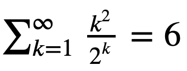
Question 11.1
Let’s verify it using summation of elements of an ndarray.
Hint: Start with the first 10 terms k = np.arange(1,11). Then try the first 30 terms.
Array broadcasting
An extremely useful feature of universal functions is the ability to operate between arrays of different sizes and shapes, a set of operations known as broadcasting.
a = np.array([0, 1, 2])    # 1D array
b = np.ones((3,3))         # 2D array
a + b          # `a` is stretched/broadcast across the 2nd dimension before addition;
               # effectively we add `a` to each row of `b`
In the following example both arrays are broadcast from 1D to 2D to match the shape of the other:
a = np.arange(3)                     # 1D row;                a.shape is (3,)
b = np.arange(3).reshape((3,1))      # effectively 1D column; b.shape is (3, 1)
a + b                                # the result is a 2D array!
NumPy’s broadcast rules are:
- the shape of an array with fewer dimensions is padded with 1’s on the left
- any array with shape equal to 1 in that dimension is stretched to match the other array’s shape
- if in any dimension the sizes disagree and neither is equal to 1, an error is raised
First example above:
********************
a: (3,)   ->  (1,3)  ->  (3,3)
b: (3,3)  ->  (3,3)  ->  (3,3)
                                ->  (3,3)
Second example above:
*********************
a: (3,)  ->  (1,3)  ->  (3,3)
b: (3,1) ->  (3,1)  ->  (3,3)
                                ->  (3,3)
Example 3:
**********
a: (2,3)  ->  (2,3)  ->  (2,3)
b: (3,)   ->  (1,3)  ->  (2,3)
                                ->  (2,3)
Example 4:
**********
a: (3,2)  ->  (3,2)  ->  (3,2)
b: (3,)   ->  (1,3)  ->  (3,3)
                                ->  error
"ValueError: operands could not be broadcast together with shapes (3,2) (3,)"
Let’s use broadcasting to plot a 2D function with matplotlib:
%matplotlib inline
import matplotlib.pyplot as plt
plt.figure(figsize=(12,12))
x = np.linspace(0, 5, 50)
y = np.linspace(0, 5, 50).reshape(50,1)
z = np.sin(x)**8 + np.cos(5+x*y)*np.cos(x)    # broadcast in action!
plt.imshow(z)
plt.colorbar(shrink=0.8)
Question `building a 3D array`
Use NumPy broadcasting to build a 3D array from three 1D ones.Question `converting velocity components`
This is a take-home exercise. Consider the following (inefficient) Python code that converts the spherical velocity components to the Cartesian velocity components on a $500\times 300\times 800$ spherical grid:
#!/usr/bin/env python
import numpy as np
from scipy.special import lpmv
import time

nlat, nr, nlon = 500, 300, 800   # 120e6 grid points

latitude = np.linspace(-90, 90, nlat)
radius = np.linspace(3485, 6371, nr)
longitude = np.linspace(0, 360, nlon)

# spherical velocity components: use Legendre Polynomials to set values
vlat = lpmv(0,3,latitude/90).reshape(nlat,1,1) + np.linspace(0,0,nr).reshape(nr,1) + np.linspace(0,0,nlon)
vrad = np.linspace(0,0,nlat).reshape(nlat,1,1) + lpmv(0,3,(radius-4928)/1443).reshape(nr,1) + np.linspace(0,0,nlon)
vlon = np.linspace(0,0,nlat).reshape(nlat,1,1) + np.linspace(0,0,nr).reshape(nr,1) + lpmv(0,2,longitude/180-1.)

# Cartesian velocity components
vx = np.zeros((nlat,nr,nlon))
vy = np.zeros((nlat,nr,nlon))
vz = np.zeros((nlat,nr,nlon))

start = time.time()
for i in range(nlat):
    for j in range(nr):
        for k in range(nlon):
            vx[i,j,k] = - np.sin(np.radians(longitude[k]))*vlon[i,j,k] \
              - np.sin(np.radians(latitude[i]))*np.cos(np.radians(longitude[k]))*vlat[i,j,k] \
              + np.cos(np.radians(latitude[i]))*np.cos(np.radians(longitude[k]))*vrad[i,j,k]
            vy[i,j,k] = np.cos(np.radians(longitude[k]))*vlon[i,j,k] \
              - np.sin(np.radians(latitude[i]))*np.sin(np.radians(longitude[k]))*vlat[i,j,k] \
              + np.cos(np.radians(latitude[i]))*np.sin(np.radians(longitude[k]))*vrad[i,j,k]
            vz[i,j,k] = np.cos(np.radians(latitude[i]))*vlat[i,j,k] \
              + np.sin(np.radians(latitude[i]))*vrad[i,j,k]
finish = time.time()
print("It took", finish - start, "seconds")
Using NumPy further, you can speed up the nested loop between the start = ... and finish = ... lines
by at least a factor of 1,000X. If you achieve a significant speedup, please
send us your solution at “training at westdri dot ca”.
Aggregate functions
Aggregate functions take an ndarray and reduce it along one (or more) axes. E.g., in 1D:
a = np.linspace(1, 2, 100)
a.mean()     # arithmetic mean
a.max()      # maximum value
a.argmax()   # index of the maximum value
a.sum()      # sum of all values
a.prod()     # product of all values
Or in 2D:
b = np.arange(25).reshape(5,5)
>>> b.sum()
300
b.sum(axis=0)   # add rows
b.sum(axis=1)   # add columns
Boolean indexing
a = np.linspace(1, 2, 100)
a < 1.5       # array of True and/or False
a[a < 1.5]    # will only return those elements that meet True condition
a[a < 1.5].shape   # there are exactly 50 such elements
a.shape
An interesting question comes up: what will happen if we apply a mask to a multi-dimensional array? How will it show incomplete rows/columns that have both True and False masks?
b = np.arange(25).reshape(5,5)   # 2D array
b > 22      # all rows are False, except for the last row [F,F,F,T,T]
b[b > 22]   # turns out we always get a 1D array with only True elements
More NumPy functionality
NumPy provides many standard linear algebra algorithms: matrix/vector products, decompositions, eigenvalues, solving linear equations, e.g.
a = np.random.randint(0, 10, size=(8,8))
b = np.arange(1,9)
x = np.linalg.solve(a, b)
x
np.allclose(np.dot(a, x),b)    # check the solution
External packages built on top of NumPy
A lot of other packages are built on top of NumPy. E.g., there is a Python package for analysis and visualization of 3D multi-resolution volumetric data called yt which is based on NumPy. Check out this visualization produced with yt.
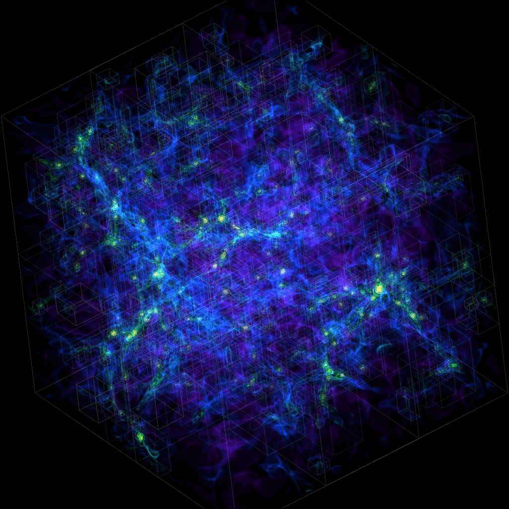
Many image-processing libraries use NumPy data structures underneath, e.g.
import skimage.io        # scikit-image is a collection of algorithms for image processing
image = skimage.io.imread(fname="https://raw.githubusercontent.com/razoumov/publish/master/grids.png")
image.shape       # it's a 1024^2 image, with (R,G,B) channels
Let’s plot this image using matplotlib:
%matplotlib inline
import matplotlib.pyplot as plt
plt.figure(figsize=(10,10))
plt.imshow(image[:,:,2], interpolation='nearest')
plt.colorbar(orientation='vertical', shrink=0.75, aspect=50)
Using NumPy, you can easily manipulate pixels:
image[:,:,2] = 255 - image[:,:,2]
and then rerun the previous (matplotlib) cell.
Another example of a package built on top of NumPy is pandas, for working with 2D tables. Going further, xarray was built on top of both NumPy and pandas. We will study pandas and xarray later in this workshop.