Setup and running Jupyter notebooks
Disclaimer: These notes started number of years ago from the official SWC lesson but then evolved quite a bit to include other topics.
Why Python?
Python is a free, open-source programming language first developed in the late 1980s and 90s that became really popular for scientific computing in the past 15 years. With Python in a few minutes you can:
- analyze thousands of texts,
- process tables with billions of records,
- manipulate thousands of images,
- restructure and process data any way you want.
Python vs. Excel
- Unlike Excel, Python can read any type of data, both structured and unstructured.
- Python is free and open-source, so no artificial limitations on where/how you run it.
- Python works on all platforms: Windows, Mac, Linux, Android, etc.
- Data manipulation is much easier in Python. There are hundreds of data processing, machine learning, and visualization libraries.
- Python can handle much larger amounts of data: limited not by Python, but by your available computing resources. In addition, Python can run at scale (in parallel) on larger systems.
- Python is more reproducible (rerun / modify the script).
Python vs. other programming languages
| Python pros | Python cons |
|---|---|
| elegant scripting language | slow (interpreted, dynamically typed) |
| easy to write and read code | uses indentation for code blocks |
| powerful, compact constructs for many tasks | |
| very popular across all fields | |
| huge number of external libraries |
Installing Python locally
Today we’ll be running Python in the cloud, so you can skip this section. I am listing these options in case you want to install Python on your computer after the workshop.
Option 1: Install Python from https://www.python.org/downloads making sure to check the option “Add Python to PATH” during the installation.
Option 2: Install Python and the packages via Anaconda from https://www.anaconda.com/download.
Option 3: Install Python via your favourite package manager, e.g. in MacOS – assuming you have
Homebrew installed – run the command brew install python.
Post-installation: Install 3rd-party Python packages in the Command Prompt / terminal via pip install <packageName>, e.g. to be able to run Python inside a Jupyter Notebook run pip install jupyter.
Starting Python
There are many ways to run Python commands:
- from a Unix shell you can start a Python shell and type commands there,
- you can launch Python scripts saved in plain text *.py files,
- you can execute Python cells inside Jupyter notebooks; the code is stored inside JSON files, displayed as HTML
Today’s setup
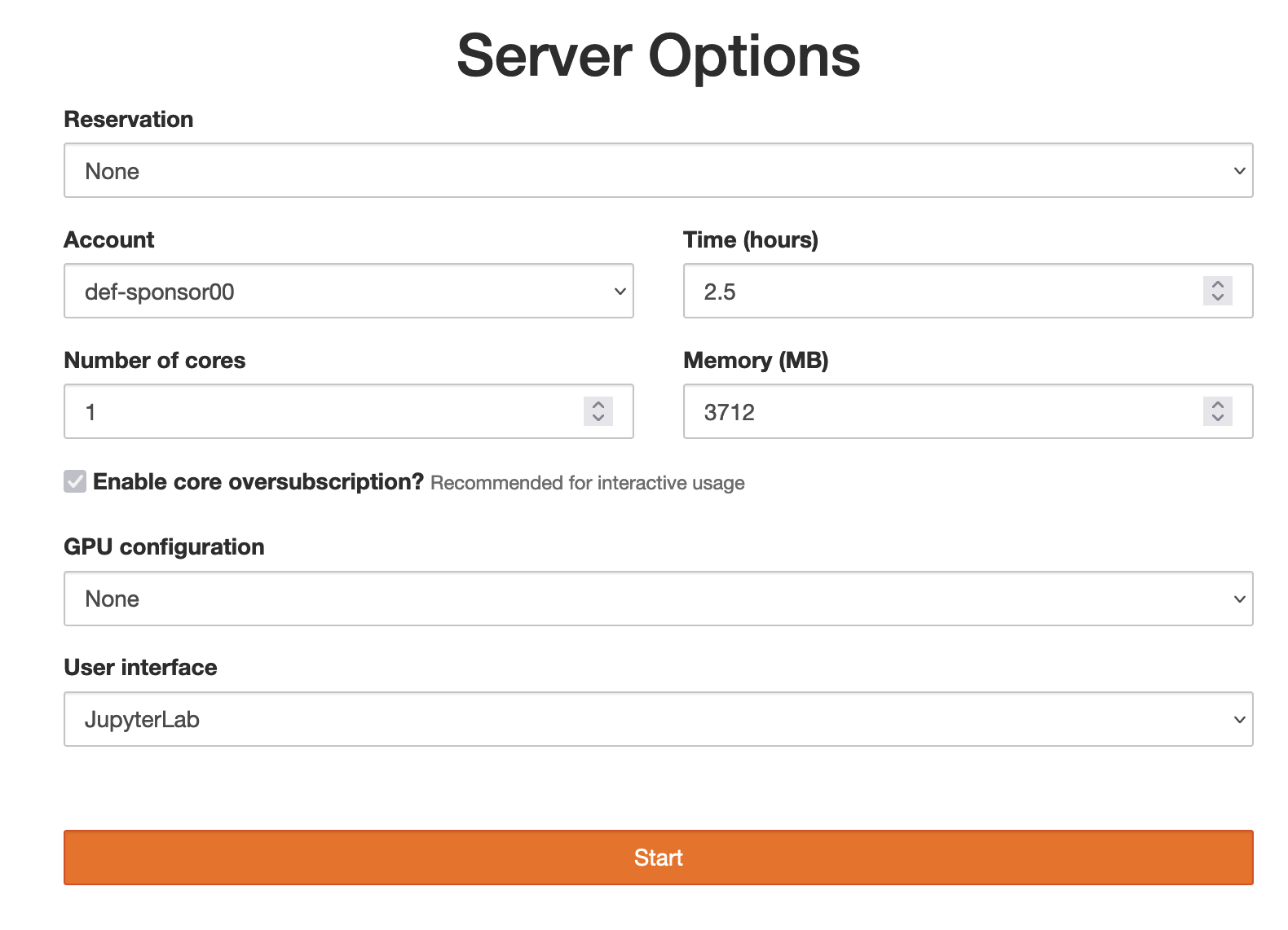
Today we’ll be using JupyterHub on our training cluster. Point your browser to https://hss.c3.ca and log in with your username and password, then launch a JupyterHub server with time = 2.5 hours, 1 CPU core, memory = 3712 MB, GPU configuration = None, user interface = JupyterLab. Finally, start a new Python 3 notebook.
After you log in, in the dashboard start a new Python 3 notebook.
Navigating Jupyter interface
- File | Save Notebook As - to rename your notebook
- File | Download - download the notebook to your computer
- File | New Launcher - to open a new launcher dashboard, e.g. to start a terminal
- File | Log Out - to terminate your job (everything is running inside a Slurm job!)
Explain: tab completion, annotating code, displaying figures inside the notebook.
- Esc - leave the cell (border changes colour) to the control mode
- A - insert a cell above the current cell
- B - insert a cell below the current cell
- X - delete the current cell
- M - turn the current cell into the markdown cell
- H - to display help
- Enter - re-enter the cell (border becomes green) from the control mode
- you can enter Latex expressions in a markdown cell, e.g. try typing
\int_0^\infty f(x)dxinside two dollar signs
print(1/2) # to run all commands in the cell, either use the Run button, or press shift+return