Parallelizing the Julia set with Base.Threads

The project is the mathematical problem to compute a Julia set – no relation to Julia language! A Julia set is defined as a set of points on the complex plane that remain bound under infinite recursive transformation $f(z)$. We will use the traditional form $f(z)=z^2+c$, where $c$ is a complex constant. Here is our algorithm:

1. pick a point $z_0\in\mathbb{C}$
2. compute iterations $z_{i+1}=z_i^2+c$ until $|z_i|>4$ (arbitrary fixed radius; here $c$ is a complex constant)
3. store the iteration number $\xi(z_0)$ at which $z_i$ reaches the circle $|z|=4$
4. limit max iterations at 255
   4.1 if $\xi(z_0)=255$, then $z_0$ is a stable point
   4.2 the quicker a point diverges, the lower its $\xi(z_0)$ is
5. plot $\xi(z_0)$ for all $z_0$ in a rectangular region $-1<=\mathfrak{Re}(z_0)<=1$, $-1<=\mathfrak{Im}(z_0)<=1$

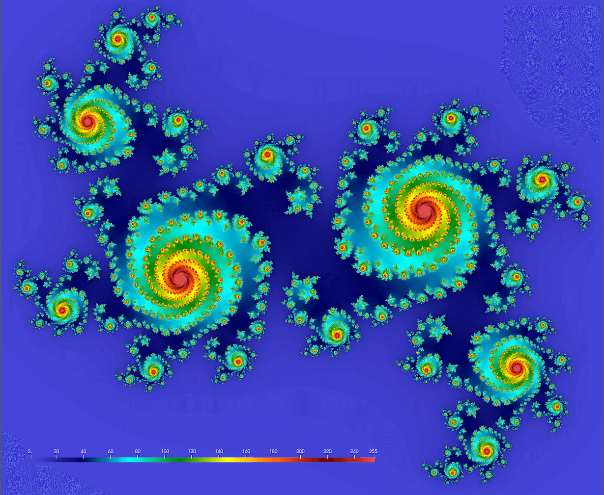
We should get something conceptually similar to this figure (here $c = 0.355 + 0.355i$; we’ll get drastically different fractals for different values of $c$):

Note: you might want to try these values too:

• $c = 1.2e^{1.1πi}$ $~\Rightarrow~$ original textbook example
• $c = -0.4-0.59i$ and 1.5X zoom-out $~\Rightarrow~$ denser spirals
• $c = 1.34-0.45i$ and 1.8X zoom-out $~\Rightarrow~$ beans
• $c = 0.34-0.05i$ and 1.2X zoom-out $~\Rightarrow~$ connected spiral boots

Below is the serial code juliaSetSerial.jl. If you are running Julia on your own computer, make sure you have the required packages:

] add BenchmarkTools
] add Plots

Let’s study the code:

using BenchmarkTools

function pixel(z)
    c = 0.355 + 0.355im
    z *= 1.2   # zoom out
    for i = 1:255
        z = z^2 + c
        if abs(z) >= 4
            return i
        end
    end
    return 255
end

const height, width = repeat([2_000],2)   # 2000^2 image

println("Computing Julia set ...")
const stability = zeros(Int32, height, width);
@btime for i in 1:height, j in 1:width
    point = (2*(j-0.5)/width-1) + (2*(i-0.5)/height-1)im # rescale to -1:1 in the complex plane
    stability[i,j] = pixel(point)
end

println("Plotting to PNG ...")
using Plots
gr()                       # initialize the gr backend
ENV["GKSwstype"] = "100"   # operate in headless mode
fname = "$(height)x$(width)"
png(heatmap(stability, size=(width,height), color=:gist_ncar), fname)

Let’s run this code with julia juliaSetSerial.jl. On my laptop it reports 931.024 ms.

function juliaSet(height, width)
    stability = zeros(Int32, height, width);
    for i in 1:height, j in 1:width
        point = (2*(j-0.5)/width-1) + (2*(i-0.5)/height-1)im # rescale to -1:1 in the complex plane
        stability[i,j] = pixel(point)
    end
end
println("Computing Julia set ...")
@btime juliaSet(2000, 2000)

println("Writing NetCDF ...")
using NetCDF
filename = "test.nc"
isfile(filename) && rm(filename)
nccreate(filename, "stability", "x", collect(1:height), "y", collect(1:width), t=NC_INT, mode=NC_NETCDF4, compress=9);
ncwrite(stability, filename, "stability");

This code will produce the file test.nc that you can download to your computer and render with ParaView or other visualization tool.

Exercise “Fractal.1”

Try one of these:

1. With NetCDF output, compare the expected and actual file sizes.
2. Try other values of the parameter $c$ (see above).
3. Increase the problem size from the default $2000^2$. Will you have enough physical memory for $8000^2$? How does this affect the runtime?

If computing takes forever, recall that @btime runs the code multiple times, while @time does it only once. Also, you might like a progress bar inside the terminal:

using ProgressMeter
@showprogress <for loop>

Parallelizing

1. Load Base.Threads.
2. Add @threads before the outer loop, and time this parallel loop.

On my laptop with 8 threads the timing is 193.942 ms (4.8X speedup) which is good but not great – certainly worse than linear speedup … The speedup on the training cluster is not great either. There could be several potential problems:

1. False sharing effect (cache issues with multiple threads writing into adjacent array elements).
2. Less than perfect load balancing between different threads.
3. Row-major vs. column-major loop order for filling in the stability array.
4. Some CPU cores are lower efficiency, and they are slowing down the whole calculation.

Take-home exercise “Fractal.2”

How would you fix this issue? If you manage to get close to 100% parallel efficiency with Base.Threads on multiple cores, we would love to see your solution! Please only check the solution once you have worked on the problem yourself.

Take-home exercise “Fractal.3”

Build a 3D cube based on the Julia set where the 3rd axis would be a slowly varying c constant. For example, try to interpolate linearly between $c = 0.355 + 0.355i$ and $c = 1.34-0.45i$, or between any other two complex values. Send us an animation traversing your volume once you are done. What highest cube resolution could you compute?