Shared and distributed arrays in Julia

Thursday, December 9, 2021
2:00pm - 4:00pm Pacific Time

This workshop is a followup to our Oct-14 introductory session on multiprocessing in Julia. Today we will take a more detailed look at DistributedArrays.jl and SharedArrays.jl that enable parallel work with large arrays. We will demo these packages using a fractal Julia set (no relation to Julia language).

Please check the notes from the previous workshop on running Julia in REPL on the training cluster.

DistributedArrays.jl

DistributedArrays package provides DArray object that can be split across several processes (set of workers), either on the same or multiple nodes. This allows use of arrays that are too large to fit in memory on one node. Each process operates on the part of the array that it owns – this provides a very natural way to achieve parallelism for large problems.

• Each worker can read any elements using their global indices
• Each worker can write only to the part that it owns $~\Rightarrow~$ automatic parallelism and safe execution

DistributedArrays is not part of the standard library, so usually you need to install it yourself (it will typically write into ~/.julia/environments/versionNumber directory):

] add DistributedArrays

We need to load DistributedArrays on every worker:

using Distributed
addprocs(4)
@everywhere using DistributedArrays

n = 10
data = dzeros(Float32, n, n);          # distributed 2D array of 0's
data                                   # can access the entire array
data[1,1], data[n,5]                   # can use global indices
data.dims                              # global dimensions (10, 10)
data[1,1] = 1.0                        # error: cannot write from the control process!
@spawnat 2 data.localpart[1,1] = 1.5   # success: can write locally
data

Let’s check data distribution across workers:

for i in workers()
    @spawnat i println(localindices(data))
end

rows, cols = @fetchfrom 3 localindices(data)
println(rows)     # the rows owned by worker 3

We can only write into data from its “owner” workers using local indices on these workers:

@everywhere function fillLocalBlock(data)
    h, w = localindices(data)
    for iGlobal in h                         # or collect(h)
        iLoc = iGlobal - h.start + 1         # always starts from 1
        for jGlobal in w                     # or collect(w)
            jLoc = jGlobal - w.start + 1     # always starts from 1
            data.localpart[iLoc,jLoc] = iGlobal + jGlobal
        end
    end
end

for i in workers()
    @spawnat i fillLocalBlock(data)
end
data   # now the distributed array is filled
@fetchfrom 3 data.localpart    # stored on worker 3
minimum(data), maximum(data)   # parallel reduction

One-liners to generate distributed arrays:

a = dzeros(100,100,100);      # 100^3 distributed array of 0's
b = dones(100,100,100);       # 100^3 distributed array of 1's
c = drand(100,100,100);       # 100^3 uniform [0,1]
d = drandn(100,100,100);      # 100^3 drawn from a Gaussian distribution
d[1:10,1:10,1]
e = dfill(1.5,100,100,100);   # 100^3 fixed value

You can find more information about the arguments by typing ?DArray. For example, you have a lot of control over the DArray’s distribution across workers. Before I show the examples, let’s define a convenient function to show the array’s distribution:

function showDistribution(x::DArray)
    for i in workers()
        @spawnat i println(localindices(x))
    end
end

nworkers()                                  # 4
data = dzeros((100,100), workers()[1:2]);   # define only on the first two workers
showDistribution(data)

square = dzeros((100,100), workers()[1:4], [2,2]);   # 2x2 decomposition
showDistribution(square)

slab = dzeros((100,100), workers()[1:4], [1,4]);   # 1x4 decomposition
showDistribution(slab)

You can take a local array and distribute it across workers:

e = fill(1.5, (10,10))   # local array
de = distribute(e)       # distribute `e` across all workers
showDistribution(de)

Exercise “DArrays.1”

Using either top or htop command on Uu, study memory usage with DistributedArrays. Are these arrays really distributed across processes? Use a largish array for this: large enough to spot memory usage, but not too large not to exceed physical memory and not to block other participants (especially if you do this on the login node).

Building a distributed array from local pieces ¹

Let’s restart Julia with julia (single control process) and load the packages:

using Distributed
addprocs(4)
using DistributedArrays       # important to load this after addprocs()
@everywhere using LinearAlgebra

We will define an 8x8 matrix with the main diagonal and two off-diagonals (tridiagonal matrix). The lines show our matrix distribution across workers:

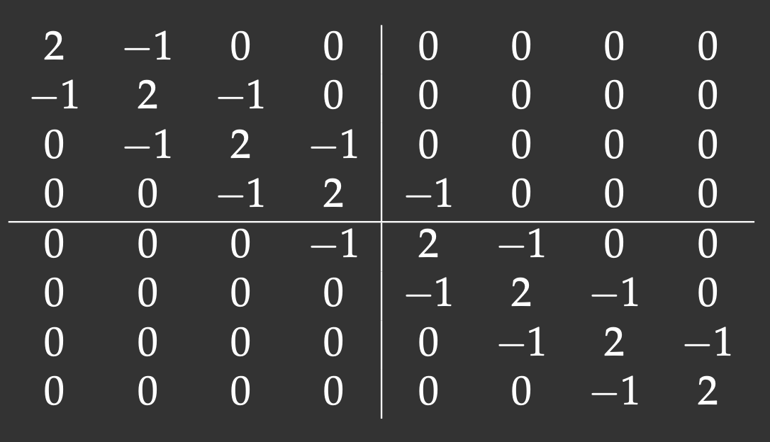
Notice that with the 2x2 decomposition two of the 4 blocks are also tridiagonal matrices. We’ll define a function to initiate them:

@everywhere function tridiagonal(n)
    la = zeros(n,n)
    la[diagind(la,0)] .= 2.     # diagind(la,k) provides indices of the kth diagonal of a matrix
    la[diagind(la,1)] .= -1.    # below the main diagonal
    la[diagind(la,-1)] .= -1.   # above the main diagonal
    return la
end

We also need functions to define the other two blocks:

@everywhere function upperRight(n)
    la = zeros(n,n)
    la[n,1] = -1.
    return la
end
@everywhere function lowerLeft(n)
    la = zeros(n,n)
    la[1,n] = -1.
    return la
end

We use these functions to define local pieces on each block and then create a distributed 8x8 matrix on a 2x2 process grid:

d11 = @spawnat 2 tridiagonal(4)
d21 = @spawnat 3 lowerLeft(4)
d12 = @spawnat 4 upperRight(4)
d22 = @spawnat 5 tridiagonal(4)
d = DArray(reshape([d11 d21 d12 d22],(2,2)))   # create a distributed 8x8 matrix on a 2x2 process grid
d

Exercise “DArrays.2”

Redefine showDistribution() on the control process and run showDistribution(d).

Running via Slurm jobs

#!/bin/bash
#SBATCH --ntasks=...   # number of MPI tasks
#SBATCH --mem-per-cpu=3600M
#SBATCH --time=0:5:0
module load julia
echo $SLURM_NODELIST
julia -p $SLURM_NTASKS code.jl   # comment out addprocs() in the code

Parallelizing Julia set

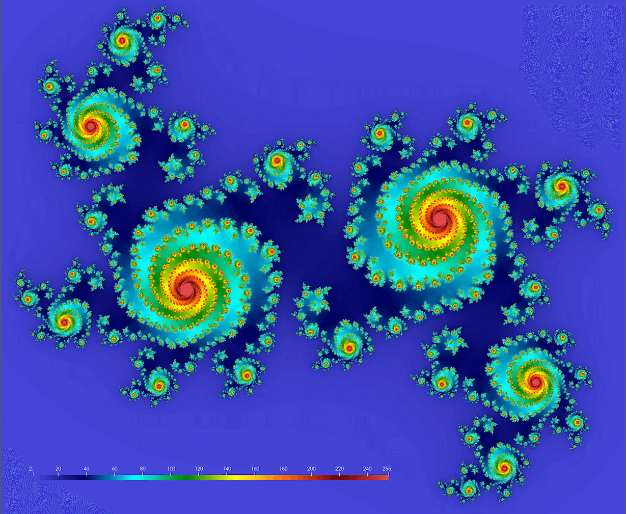
This project is the mathematical problem to compute Julia set – no relation to Julia language! A Julia set is defined as a set of points on the complex plane that remain bound under infinite recursive transformation $f(z)$. We will use the traditional form $f(z)=z^2+c$, where $c$ is a complex constant. Here is our algorithm:

1. pick a point $z_0\in\mathbb{C}$
2. compute iterations $z_{i+1}=z_i^2+c$ until $|z_i|>4$ (arbitrary fixed radius; here $c$ is a complex constant)
3. store the iteration number $\xi(z_0)$ at which $z_i$ reaches the circle $|z|=4$
4. limit max iterations at 255
   4.1 if $\xi(z_0)=255$, then $z_0$ is a stable point
   4.2 the quicker a point diverges, the lower its $\xi(z_0)$ is
5. plot $\xi(z_0)$ for all $z_0$ in a rectangular region $-1<=\mathfrak{Re}(z_0)<=1$, $-1<=\mathfrak{Im}(z_0)<=1$

We should get something conceptually similar to this figure (here $c = 0.355 + 0.355i$; we’ll get drastically different fractals for different values of $c$):

Below is the serial code juliaSetSerial.jl. First, you need to install the required packages:

] add ProgressMeter
] add NetCDF

Next, let’s study the code:

using BenchmarkTools, NetCDF

function pixel(z, c)
    for i = 1:255
        z = z^2 + c
        if abs2(z) >= 16.0
            return i
        end
    end
    return 255
end

function juliaSet(data, c, zoomOut)
    height, width = size(data)
    for i in 1:height
        y = (2*(i-0.5)/height - 1)*zoomOut      # rescale to -zoomOut:zoomOut in the complex plane
        for j in 1:width
            x = (2*(j-0.5)/width - 1)*zoomOut   # rescale to -zoomOut:zoomOut in the complex plane
            @inbounds data[i,j] = pixel(x+im*y, c)
        end
    end
end

c, zoomOut = 0.355 + 0.355im, 1.2
height = width = 1000
data = Array{Float32,2}(undef, height, width);

println("Computing Julia set ...")
@btime juliaSet(data, c, zoomOut)

# println("Very slow on-screen plotting ...")
# using Plots
# plot(heatmap(data, size=(width,height), color=:Spectral))

println("Writing NetCDF ...")
filename = "test.nc"
isfile(filename) && rm(filename)   # compact if statement
nccreate(filename, "stability", "x", collect(1:height), "y", collect(1:width), t=NC_FLOAT, mode=NC_NETCDF4, compress=9);
ncwrite(data, filename, "stability");

Let’s run this code with julia juliaSetSerial.jl. It’ll produce the file test.nc that you can download to your computer and visualize with ParaView or other visualization tool.

Exercise “Fractal.1”

1. Compare the expected and actual file sizes.
2. Try other parameter values:

c, zoomOut = 0.355 + 0.355im, 1.2   # the default one: spirals
c, zoomOut = 1.2exp(1.1π*im), 1     # original textbook example
c, zoomOut = -0.4 - 0.59im, 1.5     # denser spirals
c, zoomOut = 1.34 - 0.45im, 1.8     # beans
c, zoomOut = 0.34 -0.05im, 1.2      # connected spiral boots

3. You can also try increasing problem sizes up from $1000^2$. Will you have enough physical memory for $8000^2$? How does this affect the runtime?

Parallelizing

How would we parallelize this problem? We have a large array, so we can use DistributedArrays and compute it in parallel. Here are the steps:

1. data array should be distributed:

data = dzeros(Float32, height, width);   # distributed 2D array of 0's`

2. You need to replace juliaSet(data, c, zoomOut) with fillLocalBlock(data, c, zoomOut) to compute local pieces of data on each worker in parallel. If you don’t know where to start in this project, begin with checking the complete example with fillLocalBlock() from the previous section.
3. Functions pixel() and fillLocalBlock() should be defined on all processes.
4. Load Distributed on the control process.
5. Load DistributedArrays on all processes.
6. Replace

@btime juliaSet(data, c, zoomOut)

with

@btime @sync for i in workers()
    @spawnat i fillLocalBlock(data, c, zoomOut)
end

5. Why do we need @sync in the previous for block?
6. To the best of my knowledge, NetCDF’s ncwrite() is serial in Julia. Is there a parallel version of NetCDF for Julia? If not, then unfortunately we will have to use serial NetCDF. How do we do this with distributed data?
7. Is your parallel code faster?

Results for 1000^2

Finally, here are my timings on Uu:

Lots of things here to discuss!

One could modify our parallel code to offload some computation to the control process (not just compute on workers as we do now), so that you would see speedup when running on 2 CPUs (control process + 1 worker).

SharedArrays.jl

Unlike distributed DArray from DistributedArrays.jl, a SharedArray object is stored in full on the control process, but it is shared across all workers on the same node, with a significant cache on each worker. SharedArrays package is part of Julia’s Standard Library (comes with the language).

• Similar to DistributedArrays, you can read elements using their global indices from any worker.
• Unlike with DistributedArrays, with SharedArrays you can write into any part of the array from any worker using their global indices. This makes it very easy to parallelize any serial code.

There are certain downsides to SharedArray (compared to DistributedArrays.jl):

1. The ability to write into the same array elements from multiple processes creates the potential for a race condition and indeterministic outcome with a poorly written code!
2. You are limited to a set of workers on the same node (due to SharedArray’s intrinsic implementation).
3. You will have very skewed (non-uniform across processes) memory usage.

Let’s start with serial Julia (julia) and initialize a 1D shared array:

using Distributed, SharedArrays
addprocs(4)
a = SharedArray{Float64}(30);
a[:] .= 1.0           # assign from the control process
@fetchfrom 2 sum(a)   # correct (30.0)
@fetchfrom 3 sum(a)   # correct (30.0)

@sync @spawnat 2 a[:] .= 2.0   # can assign from any worker!
@fetchfrom 3 sum(a)            # correct (60.0)

You can use a function to initialize an array, however, pay attention to the result:

b = SharedArray{Int64}((1000), init = x -> x .= 0);    # use a function to initialize `b`
b = SharedArray{Int64}((1000), init = x -> x .+= 1)   # each worker updates the entire array in-place!

Key idea: each worker runs this function!

Let’s fill each element with its corresponding myd() value:

@everywhere println(myid())     # let's use these IDs in the next function
c = SharedArray{Int64}((20), init = x -> x .= myid())   # indeterminate outcome! each time a new result

Each worker updates every element, but the order in which they do this varies from one run to another, producing indeterminate outcome.

@everywhere using SharedArrays   # otherwise `localindices` won't be found on workers
for i in workers()
    @spawnat i println(localindices(c))   # this block is assigned for processing on worker `i`
end

What we really want is each worker should fill only its assigned block (parallel init, same result every time):

c = SharedArray{Int64}((20), init = x -> x[localindices(x)] .= myid())

Another way to avoid a race condition: use parallel for loop

Let’s initialize a 2D SharedArray:

a = SharedArray{Float64}(100,100);
@distributed for i in 1:100     # parallel for loop split across all workers
    for j in 1:100
	    a[i,j] = myid()           # ID of the worker that initialized this element
    end
end
for i in workers()
    @spawnat i println(localindices(a))   # weird: shows 1D indices for 2D array
end
a                           # available on all workers
a[1:10,1:10]                # on the control process
@fetchfrom 2 a[1:10,1:10]   # on worker 2