Using libraries from Python
https://wgpages.netlify.app/pythonlibraries
Thursday, January 26
10:30am - 5:00pm
Instructors: Marie-Helene Burle & Alex Razoumov (SFU)
Target audience: general
Level: beginner
Prerequisites: first half of today’s workshop – the notes can be found here .
Part 2: libraries intro
Most of the power of a programming language is in its libraries. This is especially true for Python which is an interpreted language and is therefore very slow (compared to compiled languages). However, the libraries are often compiled (can be written in compiled languages such as C/C++) and therefore offer much faster performance than native Python code.
A library is a collection of functions that can be used by other programs. Python’s standard library includes many functions we worked with before (print, int, round, …) and is included with Python. There are many other additional modules in the standard library such as math:
print('pi is', pi)
import math
print('pi is', math.pi)
You can also import math’s items directly:
from math import pi, sin
print('pi is', pi)
sin(pi/6)
cos(pi)
help(math)   # help for libraries works just like help for functions
from math import *
You can also create an alias from the library:
import math as m
print m.pi
Question 8
What function from the math library can you use to calculate a square root without usingsqrt?
Question 9
You want to select a random character from the stringbases='ACTTGCTTGAC'. What standard library would you most expect
to help? Which function would you select from that library? Are there alternatives?
Question 10
A colleague of yours typeshelp(math) and gets an error: NameError: name 'math' is not defined. What has your
colleague forgotten to do?
Question 11
Convert the angle 0.3 rad to degrees using the math library.Virtual environments and packaging
To install a package into the current Python environment from inside a Jupyter notebook, simply do (you will probably need to restart the kernel before you can use the package):
%pip install packageName # e.g. try bson
In Python you can create an isolated environment for each project, into which all of its dependencies will be installed. This could be useful if your several projects have very different sets of dependencies. On the computer running your Jupyter notebooks, open the terminal and type:
(Important: on a cluster you must do this on the login node, not inside the JupyterLab terminal.)
module load python/3.9.6    # specific to HPC clusters
pip install virtualenv
virtualenv --no-download climate   # create a new virtual environment in your current directory
source climate/bin/activate
which python && which pip
pip install --no-index netcdf4 ...
pip install --no-index ipykernel    # install ipykernel (IPython kernel for Jupyter) into this environment
python -m ipykernel install --user --name=climate --display-name "My climate project"   # add your environment to Jupyter
...
deactivate
Quit all your currently running Jupyter notebooks and the Jupyter dashboard. If running on syzygy.ca, logout from your session and then log back in.
Whether running locally or on syzygy.ca, open the notebook dashboard, and one of the options in New below Python 3
should be climate.
To delete the environment, in the terminal type:
jupyter kernelspec list                  # `climate` should be one of them
jupyter kernelspec uninstall climate     # remove your environment from Jupyter
/bin/rm -rf climate
Quick overview of some of the libraries
pandasis a library for working with 2D tables / spreadsheetsnumpyis a library for working with large, multi-dimensional arrays, along with a large collection of linear algebra functions- provides missing uniform collections (arrays) in Python, along with a large number of ways to quickly process these collections ⮕ great for speeding up calculations in Python
matplotlibandplotlyare two plotting packages for Pythonscikit-imageis a collection of algorithms for image processingxarrayis a library for working with labelled multi-dimensional arrays and datasets in Python- “
pandasfor multi-dimensional arrays” - great for large scientific datasets; writes into NetCDF files
- “
Numpy
As you saw before, Python is not statically typed, i.e. variables can change their type on the fly:
a = 5
a = 'apple'
print(a)
This makes Python very flexible. Out of these variables you form 1D lists, and these can be inhomogeneous:
a = [1, 2, 'Vancouver', ['Earth', 'Moon'], {'list': 'an ordered collection of values'}]
a[1] = 'Sun'
a
Python lists are very general and flexible, which is great for high-level programming, but it comes at a cost. The Python interpreter can’t make any assumptions about what will come next in a list, so it treats everything as a generic object with its own type and size. As lists get longer, eventually performance takes a hit.
Python does not have any mechanism for a uniform/homogeneous list, where – to jump to element #1000 – you just take
the memory address of the very first element and then increment it by (element size in bytes) x 999. Numpy library
fills this gap by adding the concept of homogenous collections to python – numpy.ndarrays – which are
multidimensional, homogeneous arrays of fixed-size items (most commonly numbers).
- This brings large performance benefits!
- no reading of extra bits (type, size, reference count)
- no type checking
- contiguous allocation in memory
- numpy lets you work with mathematical arrays.
Lists and numpy arrays behave very differently:
a = [1, 2, 3, 4]
b = [5, 6, 7, 8]
a + b              # this will concatenate two lists: [1,2,3,4,5,6,7,8]
import numpy as np
na = np.array([1, 2, 3, 4])
nb = np.array([5, 6, 7, 8])
na + nb            # this will sum two vectors element-wise: array([6,8,10,12])
na * nb            # element-wise product
Working with mathematical arrays in numpy
Numpy arrays have the following attributes:
ndim= the number of dimensionsshape= a tuple giving the sizes of the dimensionssize= the total number of elementsdtype= the data typeitemsize= the size (bytes) of individual elementsnbytes= the total memory (bytes) occupied by the ndarraystrides= tuple of bytes to step in each dimension when traversing an arraydata= memory address of the array
a = np.arange(10)      # 10 integer elements 0..9
a.ndim      # 1
a.shape     # (10,)
a.nbytes    # 80
a.dtype     # dtype('int64')
b = np.arange(10, dtype=np.float)
b.dtype     # dtype('float64')
In numpy there are many ways to create arrays:
np.arange(11,20)               # 9 integer elements 11..19
np.linspace(0, 1, 100)         # 100 numbers uniformly spaced between 0 and 1 (inclusive)
np.linspace(0, 1, 100).shape
np.zeros(100, dtype=np.int)    # 1D array of 100 integer zeros
np.zeros((5, 5), dtype=np.float64)     # 2D 5x5 array of floating zeros
np.ones((3,3,4), dtype=np.float64)     # 3D 3x3x4 array of floating ones
np.eye(5)            # 2D 5x5 identity/unit matrix (with ones along the main diagonal)
You can create random arrays:
np.random.randint(0, 10, size=(4,5))    # 4x5 array of random integers in the half-open interval [0,10)
np.random.random(size=(4,3))            # 4x3 array of random floats in the half-open interval [0.,1.)
np.random.rand(3, 3)       # 3x3 array drawn from a uniform [0,1) distribution
np.random.randn(3, 3)      # 3x3 array drawn from a normal (Gaussian with x0=0, sigma=1) distribution
Indexing, slicing, and reshaping
For 1D arrays:
a = np.linspace(0,1,100)
a[0]        # first element
a[-2]       # 2nd to last element
a[5:12]     # values [5..12), also a numpy array
a[5:12:3]   # every 3rd element in [5..12), i.e. elements 5,8,11
a[::-1]     # array reversed
Similarly, for multi-dimensional arrays:
b = np.reshape(np.arange(100),(10,10))      # form a 10x10 array from 1D array
b[0:2,1]      # first two rows, second column
b[:,-1]       # last column
b[-1,:]       # last row
b[5:7,5:7]    # 2x2 block
Consider two rows:
a = np.array([1, 2, 3, 4])
b = np.array([4, 3, 2, 1])
np.vstack((a,b))   # stack them vertically into a 2x4 array (use a,b as rows)
np.hstack((a,b))   # stack them horizontally into a 1x8 array
np.column_stack((a,b))         # use a,b as columns
np.vstack((a,b)).transpose()   # same result
Vectorized functions on array elements (a.k.a. universal functions = ufunc)
One of the big reasons for using numpy is so you can do fast numerical operations on a large number of elements. The
result is another ndarray. In many calculations you can use replace the usual for/while loops with functions on
numpy elements.
a = np.arange(100)
a**2          # each element is a square of the corresponding element of a
np.log10(a+1)     # apply this operation to each element
(a**2+a)/(a+1)    # the result should effectively be a floating-version copy of a
np.arange(10) / np.arange(1,11)  # this is np.array([ 0/1, 1/2, 2/3, 3/4, ..., 9/10 ])
Consider the series 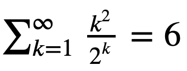
Question 11aa
Let’s verify it using summation of elements of an ndarray.
Hint: Start with the first 10 terms k = np.arange(1,11). Then try the first 30 terms.
Array broadcasting
An extremely useful feature of ufuncs is the ability to operate between arrays of different sizes and shapes, a set of operations known as broadcasting.
a = np.array([0, 1, 2])    # 1D array
b = np.ones((3,3))         # 2D array
a + b          # `a` is stretched/broadcast across the 2nd dimension before addition;
               # effectively we add `a` to each row of `b`
In the following example both arrays are broadcast from 1D to 2D to match the shape of the other:
a = np.arange(3)                     # 1D row;                a.shape is (3,)
b = np.arange(3).reshape((3,1))      # effectively 1D column; b.shape is (3, 1)
a + b                                # the result is a 2D array!
Numpy’s broadcast rules are:
- the shape of an array with fewer dimensions is padded with 1’s on the left
- any array with shape equal to 1 in that dimension is stretched to match the other array’s shape
- if in any dimension the sizes disagree and neither is equal to 1, an error is raised
First example above:
********************
a: (3,)   ->  (1,3)  ->  (3,3)
b: (3,3)  ->  (3,3)  ->  (3,3)
                                ->  (3,3)
Second example above:
*********************
a: (3,)  ->  (1,3)  ->  (3,3)
b: (3,1) ->  (3,1)  ->  (3,3)
                                ->  (3,3)
Example 3:
**********
a: (2,3)  ->  (2,3)  ->  (2,3)
b: (3,)   ->  (1,3)  ->  (2,3)
                                ->  (2,3)
Example 4:
**********
a: (3,2)  ->  (3,2)  ->  (3,2)
b: (3,)   ->  (1,3)  ->  (3,3)
                                ->  error
"ValueError: operands could not be broadcast together with shapes (3,2) (3,)"
Comment on numpy speed: Few years ago, I was working with a spherical dataset describing Earth’s mantle convection. It was defined on a spherical grid with 13e6 grid points. For each grid point, I was converting from the spherical (lateral - radial - longitudinal) velocity components to the Cartesian velocity components. For each point this is a matrix-vector multiplication. Doing this by hand with Python’s
forloops would take many hours for 13e6 points. I used numpy to vectorize in one dimension, and that cut the time to ~5 mins. At first glance, a more complex vectorization would not work, as numpy would have to figure out which dimension goes where. Writing it carefully and following the broadcast rules I made it work, with the correct solution at the end – while the total compute time went down to a couple seconds!
Let’s use broadcasting to plot a 2D function with matplotlib:
%matplotlib inline
import matplotlib.pyplot as plt
plt.figure(figsize=(12,12))
x = np.linspace(0, 5, 50)
y = np.linspace(0, 5, 50).reshape(50,1)
z = np.sin(x)**8 + np.cos(5+x*y)*np.cos(x)    # broadcast in action!
plt.imshow(z)
plt.colorbar(shrink=0.8)
Question 11ab
Use numpy broadcasting to build a 3D array from three 1D ones.Aggregate functions
Aggregate functions take an ndarray and reduce it along one (or more) axes. E.g., in 1D:
a = np.linspace(1, 2, 100)
a.mean()     # arithmetic mean
a.max()      # maximum value
a.argmax()   # index of the maximum value
a.sum()      # sum of all values
a.prod()     # product of all values
Or in 2D:
b = np.arange(25).reshape(5,5)
>>> b.sum()
300
b.sum(axis=0)   # add rows
b.sum(axis=1)   # add columns
Boolean indexing
a = np.linspace(1, 2, 100)
a < 1.5       # array of True and/or False
a[a < 1.5]    # will only return those elements that meet True condition
a[a < 1.5].shape   # there are exactly 50 such elements
a.shape
An interesting question comes up: what will happen if we apply a mask to a multi-dimensional array? How will it show incomplete rows/columns that have both True and False masks?
b = np.arange(25).reshape(5,5)   # 2D array
b > 22      # all rows are False, except for the last row [F,F,F,T,T]
b[b > 22]   # turns out we always get a 1D array with only True elements
More numpy functionality
Numpy provides many standard linear algebra algorithms: matrix/vector products, decompositions, eigenvalues, solving linear equations, e.g.
a = np.random.randint(0, 10, size=(8,8))
b = np.arange(1,9)
x = np.linalg.solve(a, b)
x
np.allclose(np.dot(a, x),b)    # check the solution
External packages built on top of numpy
A lot of other packages are built on top of numpy. E.g., there is a Python package for analysis and visualization of 3D multi-resolution volumetric data called yt which is based on numpy. Check out this visualization produced with yt.
Many image-processing libraries use numpy data structures underneath, e.g.
import skimage.io        # scikit-image is a collection of algorithms for image processing
image = skimage.io.imread(fname="https://raw.githubusercontent.com/razoumov/publish/master/grids.png")
image.shape       # it's a 1024^2 image, with (R,G,B,\alpha) channels
Let’s plot this image using matplotlib:
%matplotlib inline
import matplotlib.pyplot as plt
plt.figure(figsize=(10,10))
plt.imshow(image[:,:,2], interpolation='nearest')
plt.colorbar(orientation='vertical', shrink=0.75, aspect=50)
Using numpy, you can easily manipulate pixels:
image[:,:,2] = 255 - image[:,:,2]
and then rerun the previous (matplotlib) cell.
Another example of a package built on top of numpy is pandas, for working with 2D tables. Going further, xarray was built on top of both numpy and pandas. We will study pandas and xarray later in this workshop.
Plotting with matplotlib
Simple line/scatter plots
One of the most widely used Python plotting libraries is matplotlib. Matplotlib is open source and produces static images.
%matplotlib inline
import matplotlib.pyplot as plt
plt.figure(figsize=(10,8))
from numpy import linspace, sin
x = linspace(0.01,1,300)
y = sin(1/x)
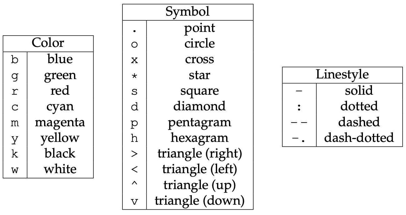
plt.plot(x, y, 'bo-')
plt.xlabel('x', fontsize=18)
plt.ylabel('f(x)', fontsize=18)
# plt.show() # not needed inside the Jupyter notebook
# plt.savefig('tmp.png')
Offscreen plotting - You can create the same plot with offscreen rendering directly to a file:
import matplotlib as mpl
import matplotlib.pyplot as plt
mpl.use('Agg')   # enable PNG backend
plt.figure(figsize=(10,8))
from numpy import linspace, sin
x = linspace(0.01,1,300)
y = sin(1/x)
plt.plot(x, y, 'bo-')
plt.xlabel('x', fontsize=18)
plt.ylabel('f(x)', fontsize=18)
plt.savefig('tmp.png')
Let’s add the second line, the labels, and the legend. Note that matplotlib automatically adjusts the axis ranges to fit both plots:
%matplotlib inline
import matplotlib.pyplot as plt
plt.figure(figsize=(10,8))
from numpy import linspace, sin
x = linspace(0.01,1,300)
y = sin(1/x)
plt.plot(x, y, 'bo-', label='one')
plt.plot(x+0.3, 2*sin(10*x), 'r-', label='two')
plt.legend(loc='lower right')
plt.xlabel('x', fontsize=18)
plt.ylabel('f(x)', fontsize=18)
Let’s plot these two functions side-by-side:
%matplotlib inline
import matplotlib.pyplot as plt
fig = plt.figure(figsize=(12,4))
from numpy import linspace, sin
x = linspace(0.01,1,300)
y = sin(1/x)

ax = fig.add_subplot(121)   # on 1x2 layout create plot #1 (`axes` object with some data space)
plt.plot(x, y, 'bo-', label='one')
ax.set_ylim(-1.5, 1.5)
plt.xlabel('x')
plt.ylabel('f1')

fig.add_subplot(122)   # on 1x2 layout create plot #2
plt.plot(x+0.2, 2*sin(10*x), 'r-', label='two')
plt.xlabel('x')
plt.ylabel('f2')
Instead of indices, we could specify the absolute coordinates of each plot with fig.add_axes():
- adjust the size
fig = plt.figure(figsize=(12,4)) - replace the first
ax = fig.add_subplot(121)withax = fig.add_axes([0.1, 0.7, 0.8, 0.3]) # left, bottom, width, height - replace the second
fig.add_subplot(122)withfig.add_axes([0.1, 0.2, 0.8, 0.4]) # left, bottom, width, height
The 3rd option for more fine-grained control is plt.axes() – it creates an axes object (a region of the figure with
some data space). These two lines are equivalent - both create a new figure with one subplot:
fig = plt.figure(figsize=(8,8)); ax = fig.add_subplot(111)
fig = plt.figure(figsize=(8,8)); ax = plt.axes()
Shortly we will see that we can pass additional flags to fig.add_subplot() and plt.axes() for more coordinate system
control.
Question 11b
Break the plot into two subplots, the fist taking 1/3 of the space on the left, the second one 2/3 of the space on the right.Let’s plot a simple line in the x-y plane:
import matplotlib.pyplot as plt
import numpy as np
fig = plt.figure(figsize=(12,12))
ax = fig.add_subplot(111)
x = np.linspace(0,1,100)
plt.plot(2*np.pi*x, x, 'b-')
plt.xlabel('x')
plt.ylabel('f1')
Replace ax = fig.add_subplot(111) with ax = fig.add_subplot(111, projection='polar'). Now we have a plot in the
phi-r plane, i.e. in polar coordinates. Phi goes [0,2\pi], whereas r goes [0,1].
?fig.add_subplot # look into `projection` parameter
import matplotlib.pyplot as plt
import numpy as np
fig = plt.figure(figsize=(12,12))
ax = fig.add_subplot(111, projection='mollweide')
x = np.radians([30,40, 50])
y = np.radians([15, 16, 17])
plt.plot(x, y, 'bo-')
You can use this projection parameter together with cartopy package to process 2D geospatial data to
produce maps, while all plotting is still being done by Matplotlib. We teach cartopy in a separate workshop.
Let’s try a scatter plot:
%matplotlib inline
import matplotlib.pyplot as plt
import numpy as np
plt.figure(figsize=(10,8))
x = np.random.random(size=1000)   # 1D array of 1000 random numbers in [0.,1.]
y = np.random.random(size=1000)
size = 1 + 50*np.random.random(size=1000)
plt.scatter(x, y, s=size, color='lightblue')
For other plot types, click on any example in the Matplotlib gallery .
For colours, see Choosing Colormaps in Matplotlib .
Heatmaps
Let’s plot a heatmap of monthly temperatures at the South Pole:
%matplotlib inline
import matplotlib.pyplot as plt
from matplotlib import cm
import numpy as np
plt.figure(figsize=(15,10))

months = ['Jan', 'Feb', 'Mar', 'Apr', 'May', 'Jun', 'Jul', 'Aug', 'Sep', 'Oct', 'Nov', 'Dec', 'Year']
recordHigh = [-14.4,-20.6,-26.7,-27.8,-25.1,-28.8,-33.9,-32.8,-29.3,-25.1,-18.9,-12.3,-12.3]
averageHigh = [-26.0,-37.9,-49.6,-53.0,-53.6,-54.5,-55.2,-54.9,-54.4,-48.4,-36.2,-26.3,-45.8]
dailyMean = [-28.4,-40.9,-53.7,-57.8,-58.0,-58.9,-59.8,-59.7,-59.1,-51.6,-38.2,-28.0,-49.5]
averageLow = [-29.6,-43.1,-56.8,-60.9,-61.5,-62.8,-63.4,-63.2,-61.7,-54.3,-40.1,-29.1,-52.2]
recordLow = [-41.1,-58.9,-71.1,-75.0,-78.3,-82.8,-80.6,-79.3,-79.4,-72.0,-55.0,-41.1,-82.8]

vlabels = ['record high', 'average high', 'daily mean', 'average low', 'record low']

Z = np.stack((recordHigh,averageHigh,dailyMean,averageLow,recordLow))
plt.imshow(Z, cmap=cm.winter)
plt.colorbar(orientation='vertical', shrink=0.45, aspect=20)
plt.xticks(range(13), months, fontsize=15)
plt.yticks(range(5), vlabels, fontsize=12)
plt.ylim(-0.5, 4.5)

for i in range(len(months)):
    for j in range(len(vlabels)):
        text = plt.text(i, j, Z[j,i],
                       ha="center", va="center", color="w", fontsize=14, weight='bold')
Question 11c
Change the text colour to black in the brightest (green) rows and columns. You can do this either by specifying rows/columns explicitly, or (better) by setting a threshold background colour.Question 11d
Modify the code to display only 4 seasons instead of the individual months.3D topographic elevation
For this we need a data file – let’s download it. Open a terminal inside your Jupyter dashboard. Inside the terminal, type:
wget http://bit.ly/pythfiles -O pfiles.zip
unzip pfiles.zip && rm pfiles.zip        # this should unpack into the directory data-python/
This will download and unpack the ZIP file into your home directory. You can now close the terminal panel. Let’s switch back to our Python notebook and check our location:
%pwd       # run `pwd` bash command
%ls        # make sure you see data-python/
Let’s plot tabulated topographic elevation data:
from mpl_toolkits.mplot3d import Axes3D
from matplotlib import cm
from matplotlib.colors import LightSource
import matplotlib.pyplot as plt
import numpy as np
import pandas as pd

table = pd.read_csv('data-python/mt_bruno_elevation.csv')
z = np.array(table)
nrows, ncols = z.shape
x = np.linspace(0,1,ncols)
y = np.linspace(0,1,nrows)
x, y = np.meshgrid(x, y)
ls = LightSource(270, 45)
rgb = ls.shade(z, cmap=cm.gist_earth, vert_exag=0.1, blend_mode='soft')

fig, ax = plt.subplots(subplot_kw=dict(projection='3d'), figsize=(10,10))    # figure with one subplot
ax.view_init(20, 30)      # (theta, phi) viewpoint
surf = ax.plot_surface(x, y, z, facecolors=rgb, linewidth=0, antialiased=False, shade=False)
Question 11e
Replacefig, ax = plt.subplots() with fig = plt.figure() followed by ax = fig.add_subplot(). Don’t forget about
the 3d projection. This one is a little tricky – feel free to google the problem.
Let’s replace the last line with the following (running this takes ~10s on my laptop):
surf = ax.plot_surface(x, y, z, facecolors=rgb, linewidth=0, antialiased=False, shade=False)
for angle in range(90):
    print(angle)
    ax.view_init(20, 30+angle)
    plt.savefig('frame%04d'%(angle)+'.png')
And then we can create a movie in bash:
ffmpeg -r 30 -i frame%04d.png -c:v libx264 -pix_fmt yuv420p -vf "scale=trunc(iw/2)*2:trunc(ih/2)*2" spin.mp4
3D parametric plot
Here is something visually very different, still using ax.plot_surface():
from mpl_toolkits.mplot3d import Axes3D
from matplotlib import cm
from matplotlib.colors import LightSource
import matplotlib.pyplot as plt
from numpy import pi, sin, cos, mgrid

dphi, dtheta = pi/250, pi/250    # 0.72 degrees
[phi, theta] = mgrid[0:pi+dphi*1.5:dphi, 0:2*pi+dtheta*1.5:dtheta]
        # define two 2D grids: both phi and theta are (252,502) numpy arrays
r = sin(4*phi)**3 + cos(2*phi)**3 + sin(6*theta)**2 + cos(6*theta)**4
x = r*sin(phi)*cos(theta)   # x is also (252,502)
y = r*cos(phi)              # y is also (252,502)
z = r*sin(phi)*sin(theta)   # z is also (252,502)

ls = LightSource(270, 45)
rgb = ls.shade(z, cmap=cm.gist_earth, vert_exag=0.1, blend_mode='soft')

fig, ax = plt.subplots(subplot_kw=dict(projection='3d'), figsize=(10,10))
ax.view_init(20, 30)
surf = ax.plot_surface(x, y, z, facecolors=rgb, linewidth=0, antialiased=False, shade=False)
Pandas dataframes
Reading tabular data into dataframes
In this section we will be reading datasets from data-python. If you have not downloaded it in the previous
section, open a terminal and type:
wget http://bit.ly/pythfiles -O pfiles.zip
unzip pfiles.zip && rm pfiles.zip        # this should unpack into the directory data-python/
You can now close the terminal panel. Let’s switch back to our Python notebook and check our location:
%pwd       # run `pwd` bash command
%ls        # make sure you see data-python/
Pandas is a widely-used Python library for working with tabular data, borrows heavily from R’s dataframes, built on top of numpy. We will be reading the data we downloaded a minute ago into a pandas dataframe:
import pandas as pd
data = pd.read_csv('data-python/gapminder_gdp_oceania.csv')
print(data)
data   # this prints out the table nicely in Jupyter Notebook!
data.shape    # shape is a *member variable inside data*
data.info()   # info is a *member method inside data*
Question 11f
Try reading a much bigger Jeopardy dataset. First, download it with:
wget https://bit.ly/3kcsQIe -O jeopardy.csv.gz && gunzip jeopardy.csv.gz
and then read it into a dataframe game. How many lines and columns does it have?
Use dir(data) to list all member variables and methods. Then call one of them without (), and if it’s a
method it’ll tell you, so you’ll need to use ().
Rows are observations, and columns are the observed variables. You can add new observations at any time.
Currently the rows are indexed by number. Let’s index by country:
data = pd.read_csv('data-python/gapminder_gdp_oceania.csv', index_col='country')
data
data.shape     # now 12 columns
data.info()    # it's a dataframe! show row/column names, precision, memory usage
print(data.columns)   # will list all the columns
print(data.T)   # this will transpose the dataframe; curously this is a variable
data.describe()   # will print some statistics of numerical columns (very useful for 1000s of rows!)
Question 12a
Quick question: how would you list all country names?
Hint: try data.T.columns
Question 12b
Read the data ingapminder_gdp_americas.csv (which should be in the same directory as gapminder_gdp_oceania.csv)
into a variable called americas and display its summary statistics.
Question 13
Write a command to display the first three rows of theamericas data frame. What about the last three columns of this
data frame?
Question 14
The data for your current project is stored in a file called microbes.csv, which is located in a folder called
field_data. You are doing analysis in a notebook called analysis.ipynb in a sibling folder called thesis:
your_home_directory/
+-- fieldData/
  +-- microbes.csv
+-- thesis/
  +-- analysis.ipynb
What value(s) should you pass to read_csv() to read microbes.csv in analysis.ipynb?
Question 15
As well as theread_csv() function for reading data from a file, Pandas provides a to_csv() function to write data
frames to files. Applying what you’ve learned about reading from files, write one of your data frames to a file called
processed.csv. You can use help to get information on how to use to_csv().
Subsetting
data = pd.read_csv('data-python/gapminder_gdp_europe.csv', index_col='country')
data.head()
Let’s rename the first column:
data.rename(columns={'gdpPercap_1952': 'y1952'}) # this renames only one but does not change `data`
Note: we could also name the column ‘1952’, but some Pandas operations don’t work with purely numerical column names.
Let’s go through all columns and assign the new names:
for col in data.columns:
    print(col, col[-4:])
    data = data.rename(columns={col: 'y'+col[-4:]})

data
Pandas lets you subset elements using either their numerical indices or their row/column names. Long time ago Pandas
used to have a single function to do both. Now there are two separate functions, iloc() and loc(). Let’s print one
element:
data.iloc[0,0]               # the very first element by position
data.loc['Albania','y1952']   # exactly the same; the very first element by label
Printing a row:
data.loc['Albania',:]   # usual Python's slicing notation - show all columns in that row
data.loc['Albania']     # exactly the same
data.loc['Albania',]    # exactly the same
Printing a column:
data.loc[:,'y1952']   # show all rows in that column
data['y1952']         # exactly the same; single index refers to columns
data.y1952            # most compact notation; does not work with numerical-only names
Printing a range:
data.loc['Italy':'Poland','y1952':'y1967']   # select multiple rows/columns
data.iloc[0:2,0:3]
Result of slicing can be used in further operations:
data.loc['Italy':'Poland','y1952':'y1967'].max()   # max for each column
data.loc['Italy':'Poland','y1952':'y1967'].min()   # min for each column
Use comparisons to select data based on value:
subset = data.loc['Italy':'Poland', 'y1962':'y1972']
print(subset)
print(subset > 1e4)
Use a Boolean mask to print values (meeting the condition) or NaN (not meeting the condition):
mask = (subset > 1e4)
print(mask)
print(subset[mask])   # will print numerical values only if the corresponding elements in mask are True
NaN’s are ignored by statistical operations which is handy:
subset[mask].describe()
subset[mask].max()
Question 16
Assume Pandas has been imported into your notebook and the Gapminder GDP data for Europe has been loaded:
df = pd.read_csv('data-python/gapminder_gdp_europe.csv', index_col='country')
Write an expression to find the per capita GDP of Serbia in 2007.
Question 17
Explain what each line in the following short program does, e.g. what is in the variables first, second, …:
first = pd.read_csv('data-python/gapminder_all.csv', index_col='country')
second = first[first['continent'] == 'Americas']
third = second.drop('Puerto Rico')
fourth = third.drop('continent', axis = 1)
fourth.to_csv('result.csv')
Question 18
Explain in simple terms what idxmin() and idxmax() do in the short program below. When would you use these methods?
data = pd.read_csv('data-python/gapminder_gdp_europe.csv', index_col='country')
print(data.idxmin())
print(data.idxmax())
How do you create a dataframe from scratch? Many ways; the easiest by defining columns:
col1 = [1,2,3]
col2 = [4,5,6]
pd.DataFrame({'a': col1, 'b': col2})       # dataframe from a dictionary
Let’s index the rows by hand:
pd.DataFrame({'a': col1, 'b': col2}, index=['a1','a2','a3'])
Three solutions to a classification problem
Let’s create a simple dataframe from scratch:
import pandas as pd
import numpy as np

df = pd.DataFrame()
size = 10_000
df['studentID'] = np.arange(1, size+1)
df['grade'] = np.random.choice(['A', 'B', 'C', 'D'], size)

df.head()
Let’s built a new column with an alphabetic grade based on the numeric grade column. Let’s start by processing a row:
def result(row):
    if row['grade'] == 'A':
        return 'pass'
    return 'fail'
We can apply this function to each row in a loop:
%%timeit
for index, row in df.iterrows():
    df.loc[index, 'outcome'] = result(row)
We can use df.apply() to apply this function to each row:
%%timeit
df['outcome'] = df.apply(result, axis=1)   # axis=1 applies the function to each row
Or we could use a mask to only assign pass to rows with A:
%%timeit
df['outcome'] = 'fail'
df.loc[df['grade'] == 'A', 'outcome'] = 'pass'
Looping over data sets
Let’s say we want to read several files in data-python/. We can use for to loop through their list:
for filename in ['data-python/gapminder_gdp_africa.csv', 'data-python/gapminder_gdp_asia.csv']:
    data = pd.read_csv(filename, index_col='country')
    print(filename, data.min())   # print min for each column
If we have many (10s or 100s) files, we want to specify them with a pattern:
from glob import glob
print('all csv files in data-python:', glob('data-python/*.csv'))    # returns a list
print('all text files in data-python:', glob('data-python/*.txt'))   # empty list
list = glob('data-python/*.csv')
len(list)
for filename in glob('data-python/gapminder*.csv'):
    data = pd.read_csv(filename)
    print(filename, data.gdpPercap_1952.min())
Question 19
Which of these files is not matched by the expression glob('data/*as*.csv')?
A. data/gapminder_gdp_africa.csv
B. data/gapminder_gdp_americas.csv
C. data/gapminder_gdp_asia.csv
D. 1 and 2 are not matched
Question 20
Modify this program so that it prints the number of records in the file that has the fewest records.
fewest = ____
for filename in glob('data/*.csv'):
    fewest = ____
print('smallest file has', fewest, 'records')
Multidimensional labeled arrays and datasets with xarray
Xarray library is built on top of numpy and pandas, and it brings the power of pandas to multidimensional arrays. There are two main data structures in xarray:
- xarray.DataArray is a fancy, labelled version of numpy.ndarray
- xarray.Dataset is a collection of multiple xarray.DataArray’s that share dimensions
Data array: simple example from scratch
import xarray as xr
import numpy as np
data = xr.DataArray(
    np.random.random(size=(4,3)),
    dims=("y","x"),  # dimension names (row,col); we want `y` to represent rows and `x` columns
    coords={"x": [10,11,12], "y": [10,20,30,40]}  # coordinate labels/values
)
data
type(data)   # <class 'xarray.core.dataarray.DataArray'>
We can access various attributes of this array:
data.values                 # the 2D numpy array
data.values[0,0] = 0.53     # can modify in-place
data.dims                   # ('y', 'x')
data.coords                 # all coordinates
data.coords['x']            # one coordinate
data.coords['x'][1]         # a number
data.x[1]                   # the same
Let’s add some arbitrary metadata:
data.attrs = {"author": "Alex", "date": "2020-08-26"}
data.attrs["name"] = "density"
data.attrs["units"] = "g/cm^3"
data.x.attrs["units"] = "cm"
data.y.attrs["units"] = "cm"
data.attrs    # global attributes
data          # global attributes show here as well
data.x        # only `x` attributes
Subsetting arrays
We can subset using the usual Python square brackets:
data[0,:]     # first row
data[:,-1]    # last column
In addition, xarray provides these functions:
- isel() selects by index, could be replaced by [index1] or [index1,…]
- sel() selects by value
- interp() interpolates by value
data.isel()      # same as `data`
data.isel(y=1)   # second row
data.isel(y=0, x=[-2,-1])    # first row, last two columns
data.x.dtype     # it is integer
data.sel(x=10)   # certain value of `x`
data.y           # array([10, 20, 30, 40])
data.sel(y=slice(15,30))   # only values with 15<=y<=30 (two rows)
There are aggregate functions, e.g.
meanOfEachColumn = data.mean(dim='y')    # apply mean over y
spatialMean = data.mean()
spatialMean = data.mean(dim=['x','y'])   # same
Finally, we can interpolate. However, this requires scipy library and currently throws some warnings, so use at your
own risk:
data.interp(x=10.5, y=10)    # first row, between 1st and 2nd columns
data.interp(x=10.5, y=15)    # between 1st and 2nd rows, between 1st and 2nd columns
?data.interp                 # can use different interpolation methods
Plotting
Matplotlib is integrated directly into xarray:
data.plot(size=8)                         # 2D heatmap
data.isel(x=0).plot(marker="o", size=8)   # 1D line plot
Vectorized operations
You can perform element-wise operations on xarray.DataArray like with numpy.ndarray:
data + 100                           # element-wise like numpy arrays
(data - data.mean()) / data.std()    # normalize the data
data - data[0,:]      # use numpy broadcasting => subtract first row from all rows
Split your data into multiple independent groups
data.groupby("x")   # 3 groups with labels 10, 11, 12; each column becomes a group
data.groupby("x").map(lambda v: v-v.min())   # apply separately to each group
            # from each column (fixed x) subtract the smallest value in that column
Dataset: simple example from scratch
Let’s initialize two 2D arrays with the identical dimensions:
coords = {"x": np.linspace(0,1,5), "y": np.linspace(0,1,5)}
temp = xr.DataArray(      # first 2D array
    20 + np.random.randn(5,5),
    dims=("y","x"),
    coords=coords
)
pres = xr.DataArray(       # second 2D array
    100 + 10*np.random.randn(5,5),
    dims=("y","x"),
    coords=coords
)
From these we can form a dataset:
ds = xr.Dataset({"temperature": temp, "pressure": pres,
                 "bar": ("x", 200+np.arange(5)), "pi": np.pi})
ds
As you can see, ds includes two 2D arrays on the same grid, one 1D array on x, and one number:
ds.temperature   # 2D array
ds.bar           # 1D array
ds.pi            # one element
Subsetting works the usual way:
ds.sel(x=0)     # each 2D array becomes 1D array, the 1D array becomes a number, plus a number
ds.temperature.sel(x=0)     # 'temperature' is now a 1D array
ds.temperature.sel(x=0.25, y=0.5)     # one element of `temperature`
We can save this dataset to a file:
%pip install netcdf4
ds.to_netcdf("test.nc")
new = xr.open_dataset("test.nc")   # try reading it
We can even try opening this 2D dataset in ParaView - select (y,x) and deselect Spherical.
Question 21
Recall the 2D function we plotted when we were talking about numpy’s array broadcasting. Let’s scale it to a unit square x,y∈[0,1]:
x = np.linspace(0, 1, 50)
y = np.linspace(0, 1, 50).reshape(50,1)
z = np.sin(5*x)**8 + np.cos(5+25*x*y)*np.cos(5*x)
This is will our image at z=0. Then rotate this image 90 degrees (e.g. flip x and y), and this will be our function at z=1. Now interpolate linearly between z=0 and z=1 to build a 3D function in the unit cube x,y,z∈[0,1]. Check what the function looks like at intermediate z. Write out a NetCDF file with the 3D function.
Time series data
In xarray you can work with time-dependent data. Xarray accepts pandas time formatting,
e.g. pd.to_datetime("2020-09-10") would produce a timestamp. To produce a time range, we can use:
import pandas as pd
time = pd.date_range("2000-01-01", freq="D", periods=365*3+1)    # 2000-Jan to 2002-Dec (3 full years)
time
time.shape    # 1096 days
time.month    # same length (1096), but each element is replaced by the month number
time.day      # same length (1096), but each element is replaced by the day-of-the-month
?pd.date_range
Using this time construct, let’s initialize a time-dependent dataset that contains a scalar temperature variable (no
space) mimicking seasonal change. We can do this directly without initializing an xarray.DataArray first – we just need
to specify what this temperature variable depends on:
import xarray as xr
import numpy as np
ntime = len(time)
temp = 10 + 5*np.sin((250+np.arange(ntime))/365.25*2*np.pi) + 2*np.random.randn(ntime)
ds = xr.Dataset({ "temperature": ("time", temp),        # it's 1D function of time
                  "time": time })
ds.temperature.plot(size=8)
We can do the usual subsetting:
ds.isel(time=100)   # 101st timestep
ds.sel(time="2002-12-22")
Time dependency in xarray allows resampling with a different timestep:
ds.resample(time='7D')    # 1096 times -> 157 time groups
weekly = ds.resample(time='7D').mean()     # compute mean for each group
weekly.dims
weekly.temperature.plot(size=8)
Now, let’s combine spatial and time dependency and construct a dataset containing two 2D variables (temperature and pressure) varying in time. The time dependency is baked into the coordinates of these xarray.DataArray’s and should come before the spatial coordinates:
time = pd.date_range("2020-01-01", freq="D", periods=91) # January - March 2020
ntime = len(time)
n = 100      # spatial resolution in each dimension
axis = np.linspace(0,1,n)
X, Y = np.meshgrid(axis,axis)   # 2D Cartesian meshes of x,y coordinates
initialState = (1-Y)*np.sin(np.pi*X) + Y*(np.sin(2*np.pi*X))**2
finalState =   (1-X)*np.sin(np.pi*Y) + X*(np.sin(2*np.pi*Y))**2
f = np.zeros((ntime,n,n))
for t in range(ntime):
    z = (t+0.5) / ntime   # dimensionless time from 0 to 1
    f[t,:,:] = (1-z)*initialState + z*finalState

coords = {"time": time, "x": axis, "y": axis}
temp = xr.DataArray(
    20 + f,       # this 2D array varies in time from initialState to finalState
    dims=("time","y","x"),
    coords=coords
)
pres = xr.DataArray(   # random 2D array
    100 + 10*np.random.randn(ntime,n,n),
    dims=("time","y","x"),
    coords=coords
)
ds = xr.Dataset({"temperature": temp, "pressure": pres})
ds.sel(time="2020-03-15").temperature.plot(size=8)   # temperature distribution on a specific date
ds.to_netcdf("evolution.nc")
The file evolution.nc should be 100^2 x 2 variables x 8 bytes x 91 steps = 14MB. We can load it into ParaView and play
back the pressure and temperature!
Climate and forecast (CF) NetCDF convention in spherical geometry
So far we’ve been working with datasets in Cartesian coordinates. How about spherical geometry – how do we initialize and store a dataset in spherical coordinates (longitude - latitude - elevation)? Very easy: define these coordinates and your data arrays on top, put everything into an xarray dataset, and then specify the following units:
ds.lat.attrs["units"] = "degrees_north"   # this line is important to adhere to CF convention
ds.lon.attrs["units"] = "degrees_east"    # this line is important to adhere to CF convention
Question 22
Let’s do it! Create a small (one-degree horizontal + some vertical resolution), stationary (no time dependency) dataset in spherical geometry with one 3D variable and write it tospherical.nc. Load it into ParaView to make sure the
geometry is spherical.
Working with atmospheric data
I took one of the ECCC (Environment and Climate Change Canada) historical model datasets (contains only the near-surface air temperature) published on the CMIP6 Data-Archive and reduced its size, picking only a subset of timesteps:
import xarray as xr
data = xr.open_dataset('/Users/razoumov/tmp/xarray/atmosphere/tas_Amon_CanESM5_historical_r1i1p2f1_gn_185001-201412.nc')
data.sel(time=slice('2001', '2020')).to_netcdf("tasReduced.nc")   # last 168 steps
Let’s download this file in the terminal:
wget http://bit.ly/atmosdata -O tasReduced.nc
First, quickly check this dataset in ParaView (use Dimensions = (lat,lon)).
data = xr.open_dataset('tasReduced.nc')
data   # this is a time-dependent 2D dataset: print out the metadata, coordinates, data variables
data.time   # time goes monthly from 2001-01-16 to 2014-12-16
data.tas    # metadata for the data variable (time: 168, lat: 64, lon: 128)
data.tas.shape      # (168, 64, 128) = (time, lat, lon)
data.height         # at the fixed height=2m
These five lines all produce the same result:
data.tas[0] - 273.15   # take all values in the second and third dims, convert to Celsius
data.tas[0,:] - 273.15
data.tas[0,:,:] - 273.15
data.tas.isel(time=0) - 273.15
air = data.tas.sel(time='2001-01-16') - 273.15
These two lines produce the same result (1D vector of temperatures as a function of longitude):
data.tas[0,5]
data.tas.isel(time=0, lat=5)
Check temperature variation in the last step:
air = data.tas.isel(time=-1) - 273.15   # last timestep, to celsius
air.shape    # (64, 128)
air.min(), air.max()   # -43.550903, 36.82956
Selecting data is slightly more difficult with approximate floating coordinates:
data.tas.lat
data.tas.lat.dtype
data.tas.isel(lat=0)    # the first value lat=-87.86
data.lat[0]   # print the first latitude and try to use it below
data.tas.sel(lat=-87.86379884)    # does not work due to floating precision
data.tas.sel(lat=data.lat[0])     # this works
latSlice = data.tas.sel(lat=slice(-90,-80))    # only select data in a slice lat=[-90,-80]
latSlice.shape    # (168, 3, 128) - 3 latitudes in this slice
Multiple ways to select time:
data.time[-10:]   # last ten times
air = data.tas.sel(time='2014-12-16') - 273.15    # last date
air = data.tas.sel(time='2014') - 273.15    # select everything in 2014
air.shape     # 12 steps
air.time
air = data.tas.sel(time='2014-01') - 273.15    # select everything in January 2014
Aggregate functions:
meanOverTime = data.tas.mean(dim='time') - 273.15
meanOverSpace = data.tas.mean(dim=['lat','lon']) - 273.15     # mean over space for each timestep
meanOverSpace.shape     # time series (168,)
meanOverSpace.plot(marker="o", size=8)     # calls matplotlib.pyplot.plot
Interpolate to a specific location:
victoria = data.tas.interp(lat=48.43, lon=360-123.37) - 273.15
victoria.shape   # (168,) only time
victoria.plot(marker="o", size=8)      # simple 1D plot
victoria.sel(time=slice('2001','2020')).plot(marker="o", size=8)   # zoom in on the 21st-century points, see seasonal variations
Let’s plot in 2D:
air = data.tas.isel(time=-1) - 273.15   # last timestep
air.time
air.plot(size=8)     # 2D plot, very poor resolution (lat: 64, lon: 128)
air.plot(size=8, y="lon", x="lat")     # can specify which axis is which
What if we have time-dependency in the plot? We put each frame into a separate panel:
a = data.tas[-6:] - 273.15      # last 6 timesteps => 3D dataset => which coords to use for what?
a.plot(x="lon", y="lat", col="time", col_wrap=3)
Breaking into groups and applying a function to each group:
len(data.time)     # 168 steps
data.tas.groupby("time")   # 168 groups
def standardize(x):
    return (x - x.mean()) / x.std()
standard = data.tas.groupby("time").map(standardize)   # apply this function to each group
standard.shape    # (1980, 64, 128) same shape as the original but now normalized over each group